7 Plot Options

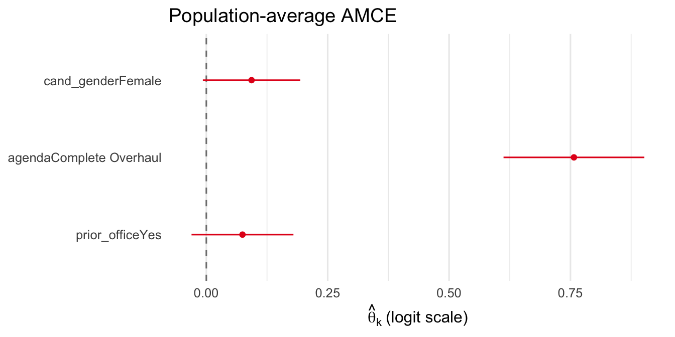
sconjoint ships six plot functions. All return plain ggplot objects that can be further customized with +. This chapter is parameter-first: it lists every customization option, grouped by purpose, and demonstrates each in isolation on a single pre-fitted object.

7.1 Plot Functions

Function	Purpose
`plot(fit, "beta_ridgelines")`	Per-respondent \(\hat\beta(Z)\) density ridgelines
`plot(fit, "loss_trace")`	Per-fold training loss curves
`plot_amce(fit)`	Population-average \(\hat\theta\) coefficient plot
`plot_fraction(fit)`	Fraction favor / oppose diverging bar chart
`plot_hetero(fit)`	Preference heterogeneity bar chart
`plot_subgroup(fit, subgroup)`	Subgroup AMCE comparison
`plot_importance(fit)`	Attribute importance ridgelines

7.2 Parameter Reference

All functions share a common set of customization parameters. Function-specific parameters are noted in parentheses.

Parameter	Applies to	Purpose	Default
`dummies`	all	Character vector: which dummies to show and in what order	`NULL` (all)
`labels`	all	Named character vector: display names for dummies	`NULL` (raw names)
`groups`	all	Named character vector: attribute group for faceting	`NULL` (no facets)
`title`	all	Main title	sensible default
`xlab` / `ylab`	all	Custom axis labels	`NULL`
`xlim`	all	Numeric(2): x-axis limits	`NULL`
`theme.bw`	all	Use `theme_bw()` instead of `theme_minimal()`	`FALSE`
`gridOff`	all	Remove grid lines	`FALSE`
`legendOff`	all	Hide the legend	`FALSE`
`legend.pos`	all	Legend position: `"bottom"`, `"right"`, `"none"`, or `c(x, y)`	varies
`cex.main`	all	Title font size multiplier	`NULL`
`cex.axis`	all	Tick label font size multiplier	`NULL`
`cex.lab`	all	Axis title font size multiplier	`NULL`
`color`	`plot_amce`	Point/line color	`"#E41A1C"`
`size` / `fatten`	`plot_amce`, `plot_subgroup`	Point size and fatten factor	`0.4` / `2`
`colors`	`plot_fraction`, `plot_subgroup`	Named color vector	defaults
`alpha` / `bar.width`	`plot_fraction`	Bar transparency and width	`0.85` / `0.65`
`gradient`	`plot_hetero`	`c(low, high)` fill gradient colors	blue scale
`sig.color` / `sig.shape`	`plot_hetero`	Marker for significant dummies	`"#B2182B"` / `18`
`dodge.width`	`plot_subgroup`	Spacing between groups	`0.6`

7.3 Selecting Variables

Use dummies to show only a subset of attribute dummies. The display order follows the order of the dummies vector.

plot_amce(fit, dummies = c("cand_genderFemale",
                            "agendaComplete Overhaul",
                            "prior_officeYes"))

This works identically across all plot functions:

plot_fraction(fit, dummies = c("cand_genderFemale",
                                "agendaComplete Overhaul"))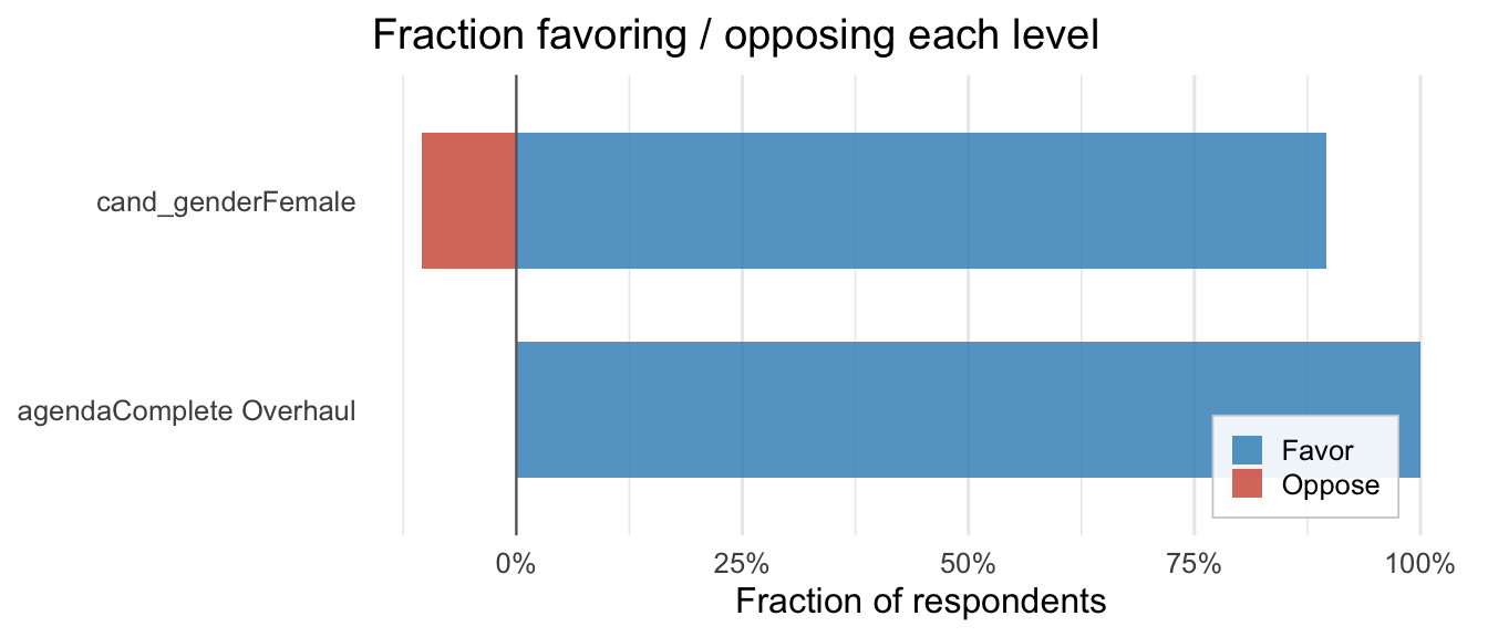

7.4 Custom Labels

Use labels to replace raw dummy names with human-readable text. Pass a named character vector; any dummy not in labels keeps its original name.

my_labels <- c(
  "agendaModerate Changes"   = "Moderate Changes",
  "agendaComplete Overhaul"  = "Complete Overhaul",
  "cand_genderFemale"        = "Female candidate",
  "prior_officeYes"          = "Prior office",
  "talentHard-Working"       = "Hard-Working",
  "talentCollaborative"      = "Collaborative"
)

plot_amce(fit, labels = my_labels)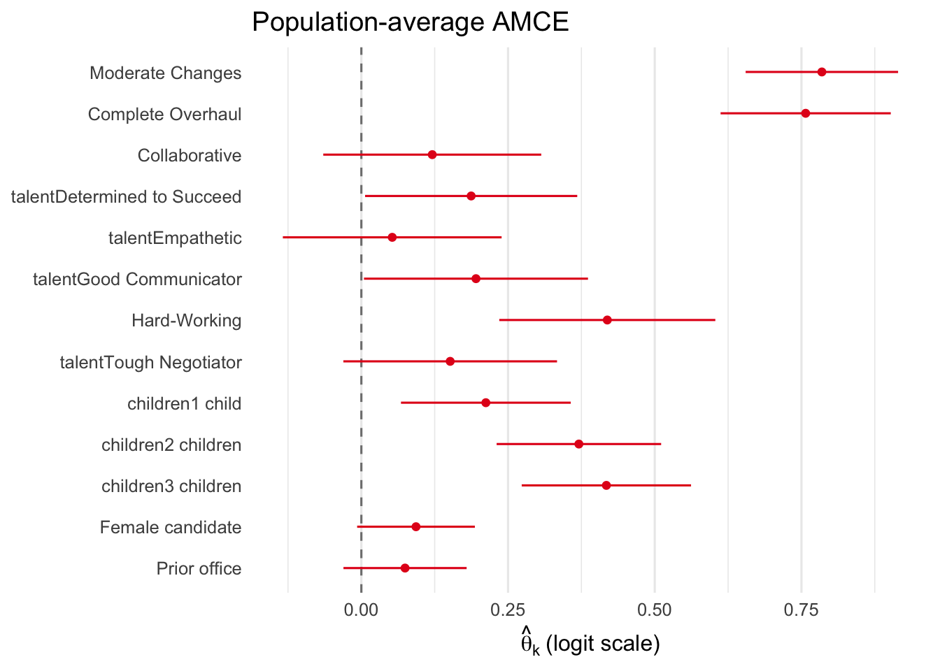

Combined with dummies for a focused, publication-ready figure:

plot_amce(fit,
          dummies = c("cand_genderFemale", "agendaComplete Overhaul"),
          labels = c("cand_genderFemale" = "Female candidate",
                     "agendaComplete Overhaul" = "Complete Overhaul"),
          title = "Key attributes")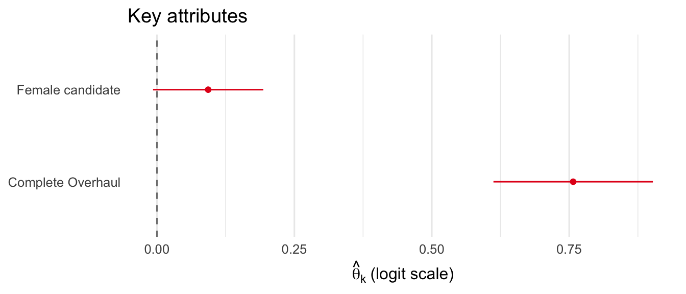

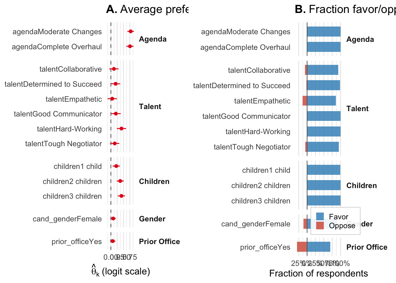
7.5 Attribute Groups

Use groups to facet the plot by attribute groups — essential for publication-quality figures.

sw_groups <- c(
  "agendaModerate Changes"  = "Agenda",
  "agendaComplete Overhaul" = "Agenda",
  "talentCollaborative"     = "Talent",
  "talentDetermined to Succeed" = "Talent",
  "talentEmpathetic"        = "Talent",
  "talentGood Communicator" = "Talent",
  "talentHard-Working"      = "Talent",
  "talentTough Negotiator"  = "Talent",
  "children1 child"         = "Children",
  "children2 children"      = "Children",
  "children3 children"      = "Children",
  "cand_genderFemale"       = "Gender",
  "prior_officeYes"         = "Prior Office"
)

plot_amce(fit, groups = sw_groups)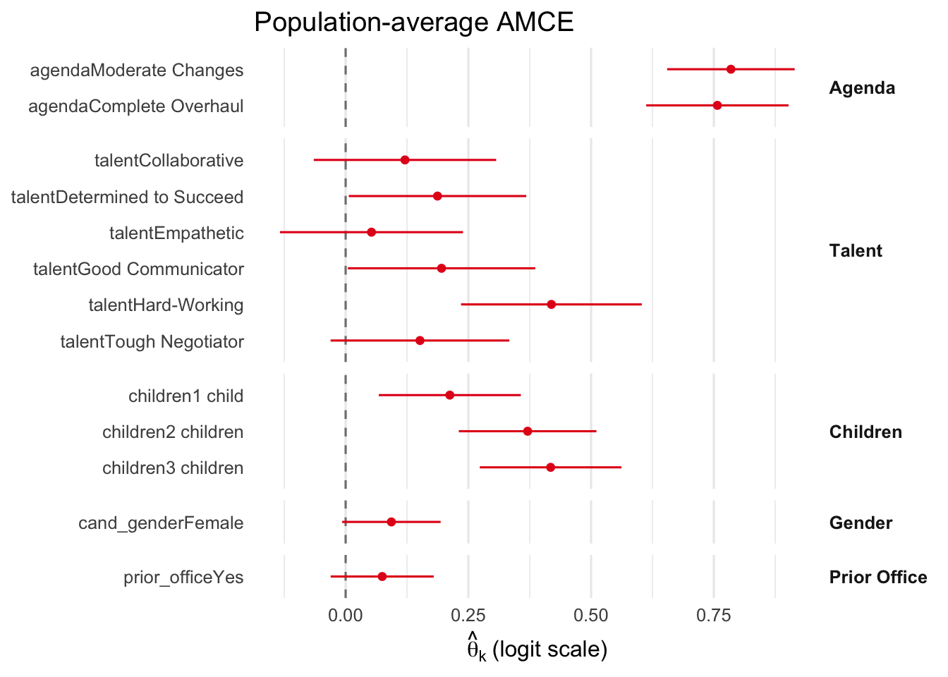

The same groups vector works across all plot functions:

plot_fraction(fit, groups = sw_groups)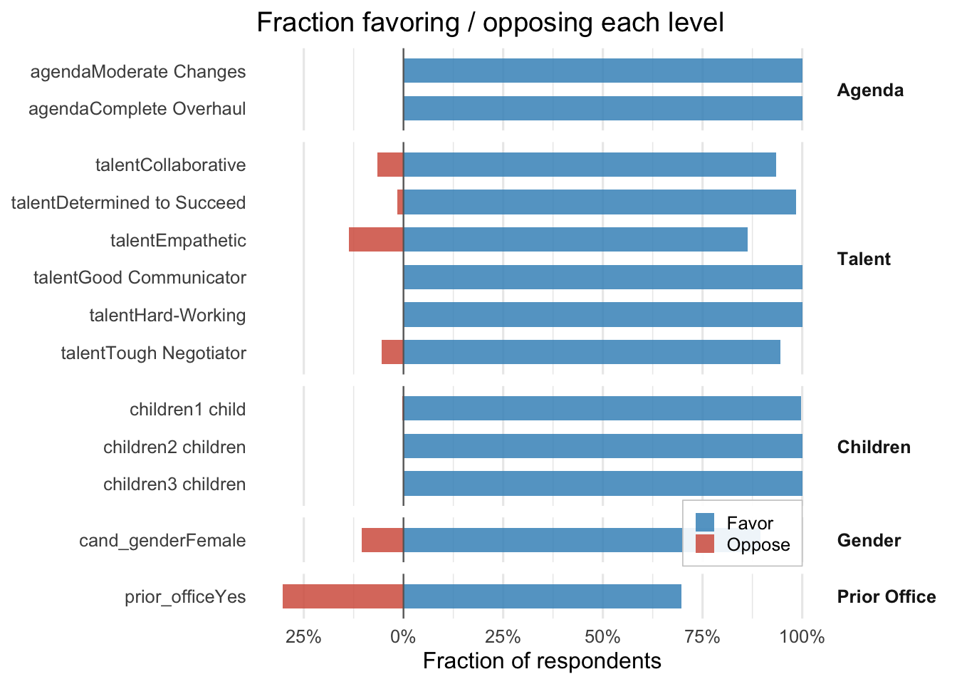

7.6 Colors

7.6.1 AMCE color

plot_amce(fit, color = "#2166AC", title = "AMCE (blue)")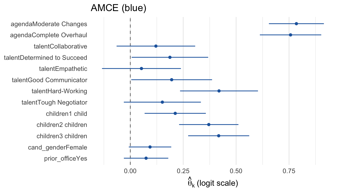

7.6.2 Fraction colors

plot_fraction(fit,
              colors = c(Favor = "#1B9E77", Oppose = "#D95F02"),
              title = "Custom fraction colors")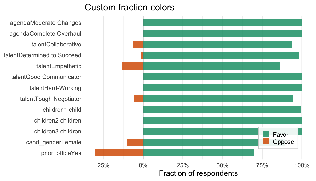

7.6.3 Heterogeneity gradient

plot_hetero(fit,
            gradient = c(low = "#FEE0D2", high = "#DE2D26"),
            sig.color = "black",
            title = "Red gradient with black markers")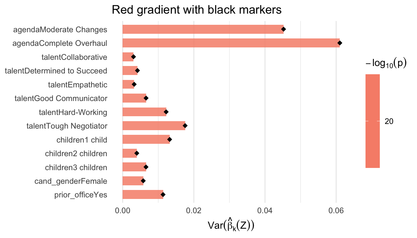

7.6.4 Subgroup colors

fem <- fit$Z[, "resp_female"] > 0.5
plot_subgroup(fit,
              subgroup = list(Female = fem, Male = !fem),
              colors = c(Female = "#7570B3", Male = "#1B9E77"),
              title = "Custom subgroup colors")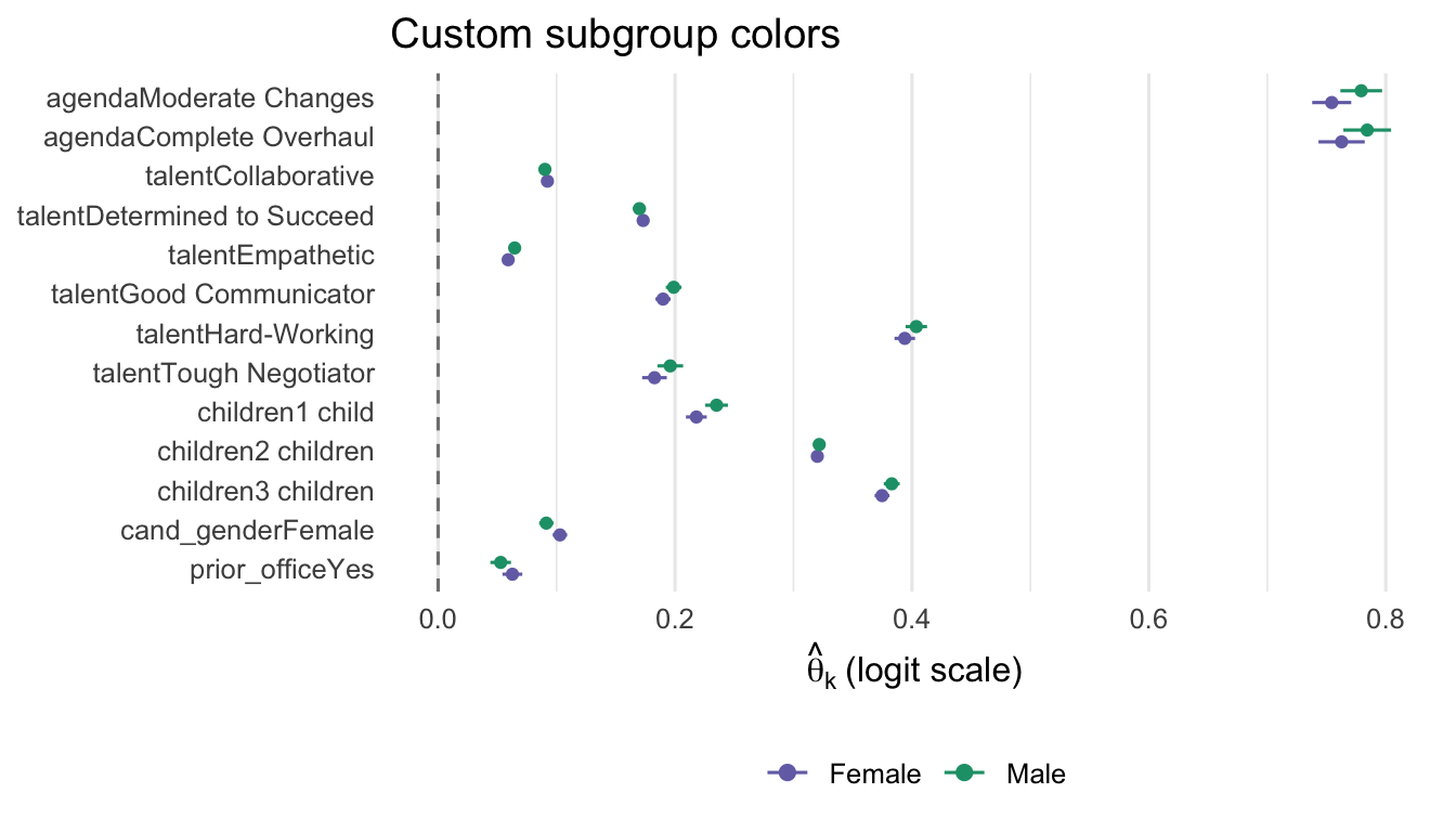

7.7 Titles and Axis Labels

plot_amce(fit,
          title = "Saha-Weeks candidate choice",
          xlab  = "Logit-scale AMCE",
          ylab  = "Attribute level")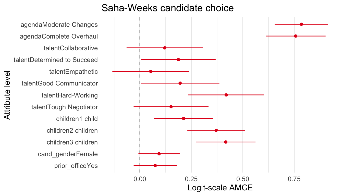

7.8 Theme and Layout

7.8.1 Black-and-white theme

plot_amce(fit, theme.bw = TRUE)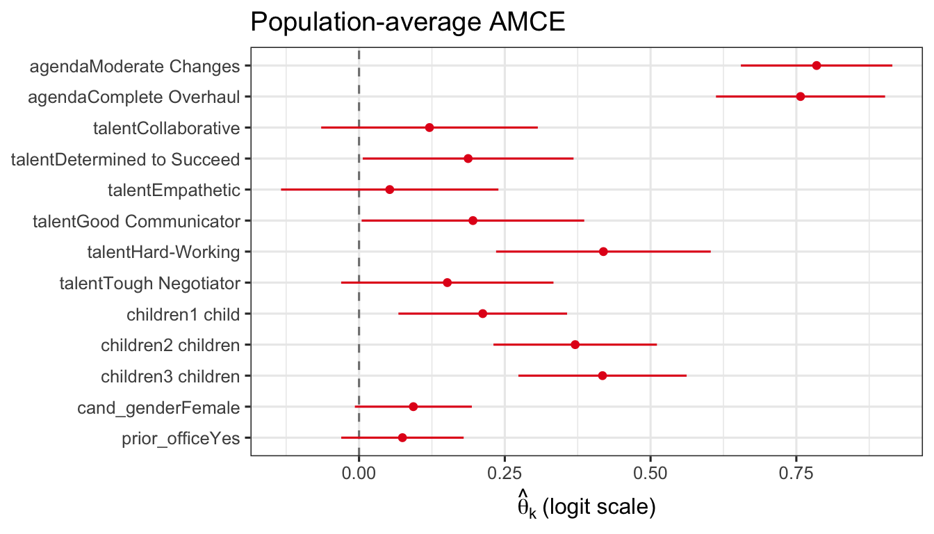

7.8.2 Remove grid lines

plot_fraction(fit, gridOff = TRUE)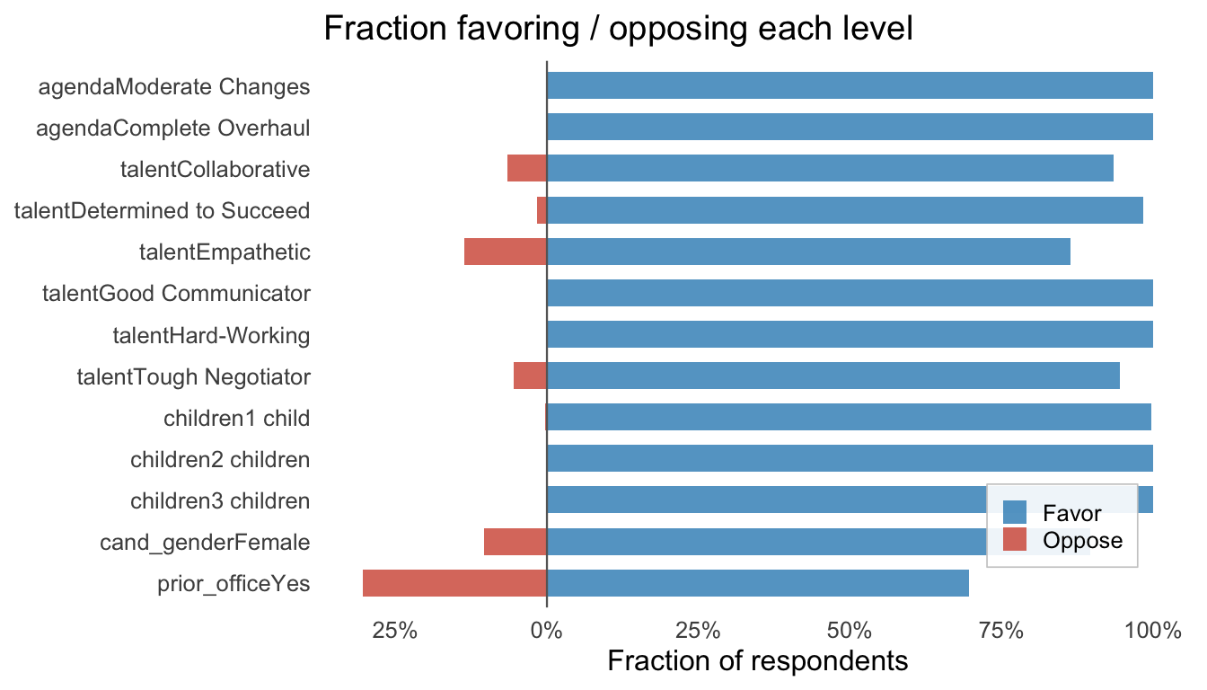

7.8.3 Font sizes

Use cex.main, cex.axis, and cex.lab as multipliers on the base font sizes (14, 11, 12 pt respectively).

plot_amce(fit, cex.main = 1.4, cex.axis = 0.9, cex.lab = 1.1)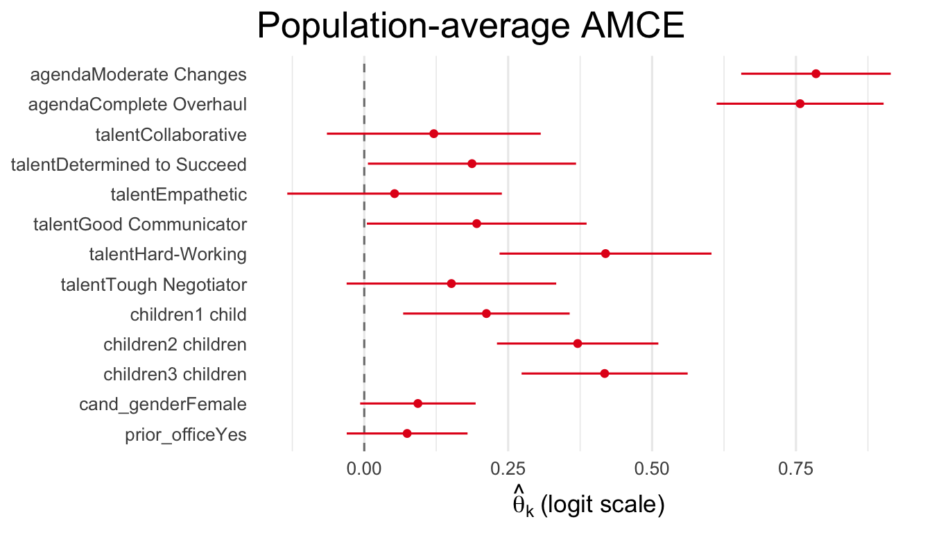

7.8.4 Legend position

fem <- fit$Z[, "resp_female"] > 0.5
plot_subgroup(fit,
              subgroup = list(Female = fem, Male = !fem),
              legend.pos = "right")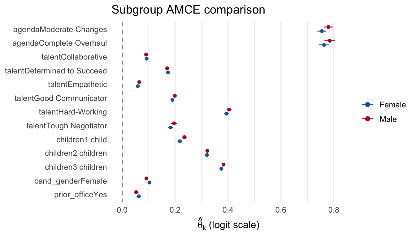

7.8.5 Hide legend

plot_fraction(fit, legendOff = TRUE)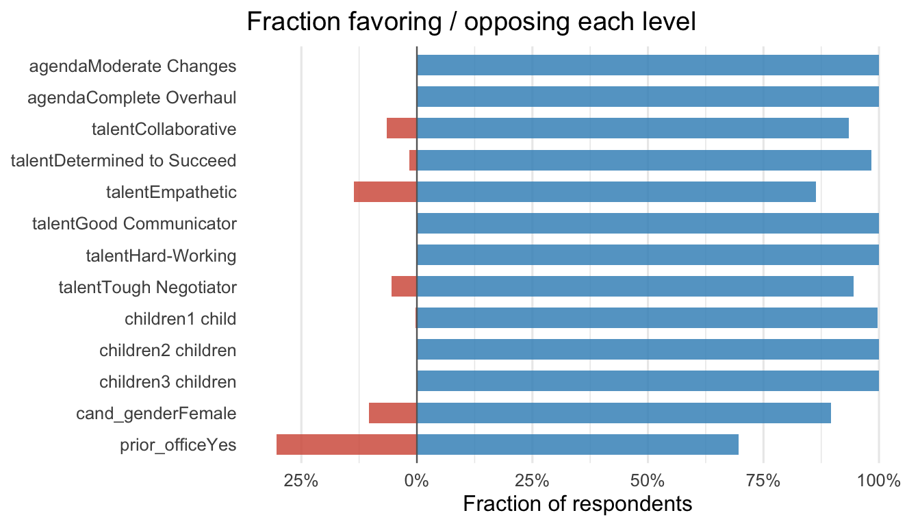

7.8.6 Axis limits

plot_amce(fit, xlim = c(-1.5, 1.5))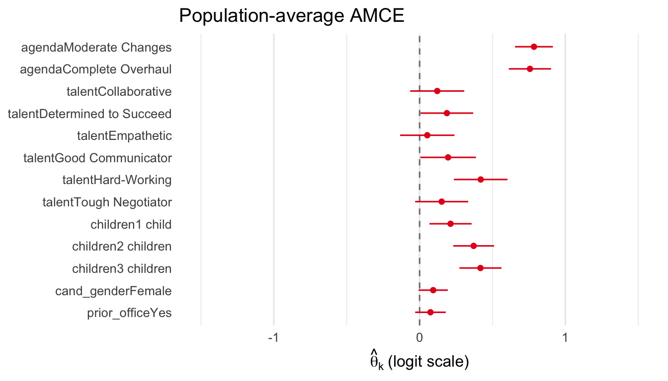

7.9 Importance

plot_importance(fit)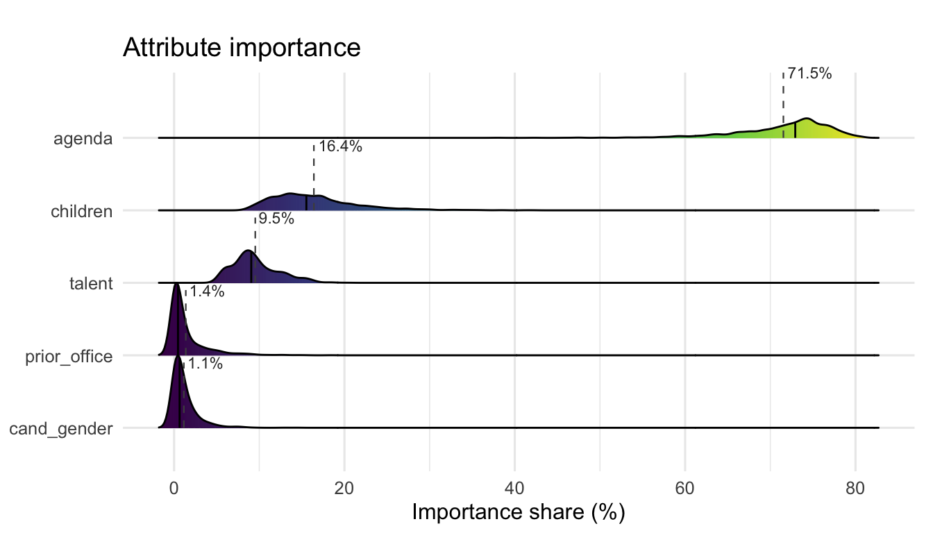

7.10 Ridgelines and Loss Trace

The plot.sc_fit() method accepts the same customization parameters via ....

plot(fit, "beta_ridgelines",
     dummies = c("agendaComplete Overhaul", "cand_genderFemale",
                  "prior_officeYes"),
     labels = c("agendaComplete Overhaul" = "Complete Overhaul",
                "cand_genderFemale" = "Female",
                "prior_officeYes" = "Prior Office"),
     title = "Selected attributes")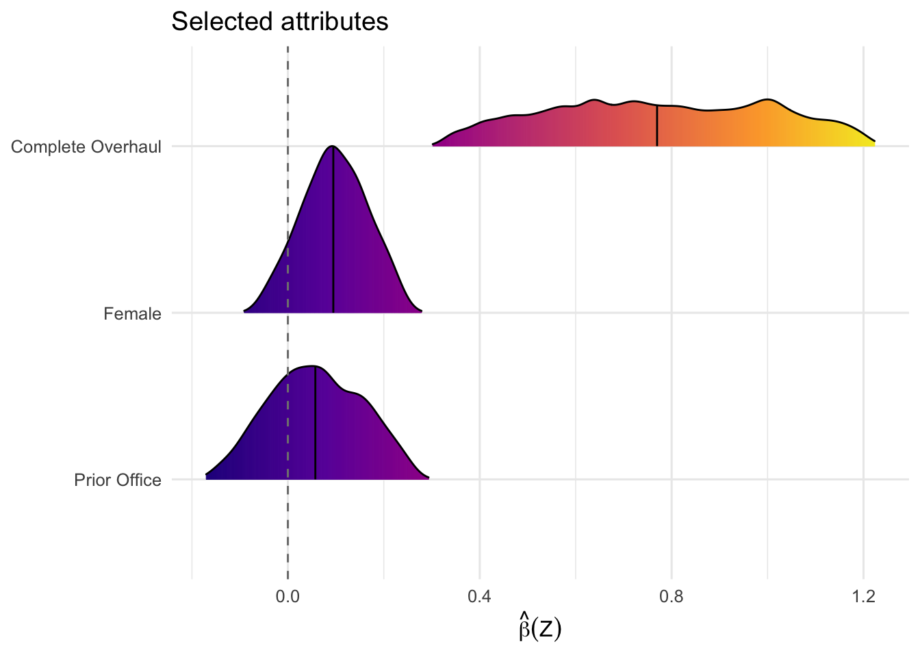

plot(fit, "loss_trace", title = "Training convergence", theme.bw = TRUE)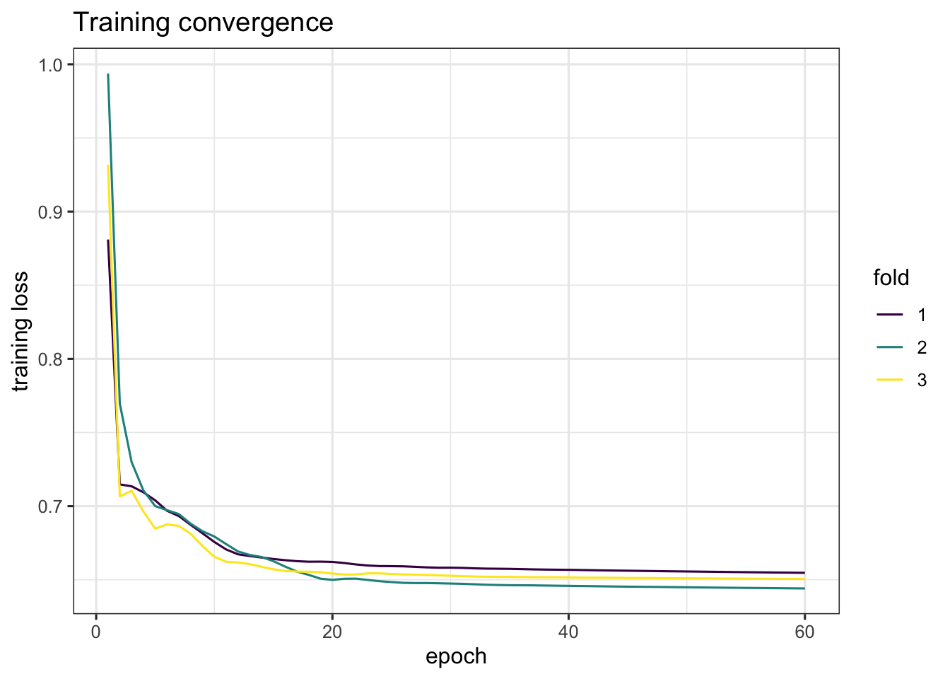

7.11 Composing with ggplot2

Since all plot functions return ggplot objects, standard ggplot2 modifications apply via +:

plot_amce(fit) +
  labs(subtitle = "Saha-Weeks (2022) candidate choice") +
  theme(plot.subtitle = element_text(color = "gray40", size = 10))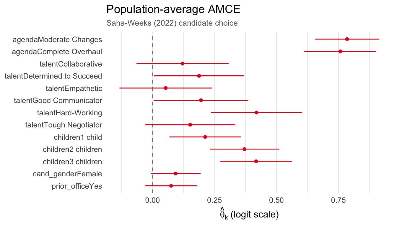

For side-by-side AMCE and fraction panels, use gridExtra:

library(gridExtra)
p1 <- plot_amce(fit, groups = sw_groups,
                title = expression(bold("A.") ~ "Average preferences"))
p2 <- plot_fraction(fit, groups = sw_groups,
                    title = expression(bold("B.") ~ "Fraction favor/oppose"))
grid.arrange(p1, p2, ncol = 2, widths = c(1, 1.1))