2  Simulated Example

Before applying the structural estimator to real data, this chapter runs the full workflow on a synthetic conjoint experiment with known ground truth. Because we control the data-generating process, every quantity the package produces can be checked against its analytically correct value.

2.1 Data-generating process

The package ships simdata, a synthetic conjoint with \(M = 1{,}000\) respondents, \(T = 6\) tasks per respondent, and two profiles per task (12,000 rows). Three binary attributes \(x_1, x_2, x_3\) are drawn independently as Bernoulli(0.5). Two continuous moderators \(z_1, z_2 \sim N(0,1)\) determine each respondent’s preference vector:

\[ \beta_1(\mathbf Z_i) = 0.5 + 0.3\,z_{1i}, \quad \beta_2(\mathbf Z_i) = -0.8 + 0.2\,z_{2i}, \quad \beta_3(\mathbf Z_i) = 0.3. \]

Key features:

  • \(\beta_1\) and \(\beta_2\) are heterogeneous (vary with \(Z\)); \(\beta_3\) is homogeneous (constant across respondents).
  • \(\beta_1 > 0\) for most respondents; \(\beta_2 < 0\) for most.
  • True population averages: \(E[\beta_1] = 0.5\), \(E[\beta_2] = -0.8\), \(E[\beta_3] = 0.3\).
data(simdata, package = "sconjoint")
dim(simdata)
[1] 12000     9
head(simdata, 6)
  respondent task profile choice x1 x2 x3       z1       z2
1          1    1       1      0  1  1  0 1.370958 2.325058
2          1    1       2      1  1  0  0 1.370958 2.325058
3          1    2       1      0  0  0  1 1.370958 2.325058
4          1    2       2      1  1  0  0 1.370958 2.325058
5          1    3       1      0  0  1  0 1.370958 2.325058
6          1    3       2      1  1  1  1 1.370958 2.325058
## True beta matrix stored as attribute
beta_true <- attr(simdata, "beta_true")
dim(beta_true)
[1] 1000    3
NoteWhy does scfit() require at least one Z column?

The DML estimator is defined in terms of a nuisance function \(\hat\beta(\mathbf Z)\) that maps respondent-level covariates into preference vectors. Without any moderators the mapping is trivial and the DML correction degenerates to a plain plug-in estimator. Users who truly want a homogeneous model should fit a standard glm(choice ~ deltaX, family = binomial) instead.

2.2 Fitting

With 1,000 respondents and 6 tasks each, the estimator has enough signal to recover both population-level and individual-level parameters cleanly.

fit_sim <- scfit(
  choice ~ x1 + x2 + x3 | z1 + z2,
  data       = simdata,
  respondent = "respondent",
  task       = "task",
  profile    = "profile",
  K          = 5L,
  n_epochs   = 200L,
  seed       = 42
)
summary(fit_sim)
sc_fit summary
Call: scfit(formula = choice ~ x1 + x2 + x3 | z1 + z2, data = simdata, 
    respondent = "respondent", task = "task", profile = "profile", 
    K = 5L, n_epochs = 200L, seed = 42)

1000 respondents | 6000 observations | K = 5 folds
hidden = 32-32-16 | epochs = 200 | seed = 42 | device = cpu

Coefficients (DML, respondent-clustered SE):
   estimate std_error z_value   p_value   ci_lo   ci_hi
x1   0.4888   0.04049  12.071 1.495e-33  0.4094  0.5682
x2  -0.8004   0.03875 -20.654 9.020e-95 -0.8764 -0.7244
x3   0.3015   0.03864   7.804 6.004e-15  0.2258  0.3772

DML/iid SE ratio (mean): 1.01

Stage 2: map_c5 | mean(sigma_prior) = 0.2902
TipHow do I know my sc_fit is well-trained?

Check two things: (1) summary(fit) reports the DML/iid SE ratio — values close to one mean the clustering correction is small and the DNN’s per-respondent \(\hat\beta\) has little additional within-respondent information beyond the population mean. (2) plot(fit, "loss_trace") shows per-fold training loss curves — they should visually level off before the last epoch. If they are still descending, increase n_epochs.

TipPerformance tips
  • Set device = "cuda" on a GPU machine; bit-exact determinism is lost but wall-clock time drops substantially.
  • Use parallel = TRUE with n_cores = parallelly::availableCores() on CPU for large datasets — the package guarantees bit-exact identity between parallel and sequential runs.
  • Prefer hidden = "auto" as a starting point and tune only when clearly needed.
plot(fit_sim, "loss_trace")

All folds converge to a similar loss level, confirming that 200 epochs is sufficient for this dataset.

2.3 Population-average recovery

The DML point estimates \(\hat\theta\) should approximate the true population means.

theta_hat <- coef(fit_sim)
theta_true <- c(x1 = 0.5, x2 = -0.8, x3 = 0.3)
data.frame(
  attribute  = names(theta_hat),
  true       = theta_true,
  estimated  = round(unname(theta_hat), 3),
  row.names  = NULL
)
  attribute true estimated
1        x1  0.5     0.489
2        x2 -0.8    -0.800
3        x3  0.3     0.302

All three signs match and the magnitudes are close. The AMCE coefficient plot makes the pattern visual:

plot_amce(fit_sim)

2.4 Individual-level recovery

The per-respondent \(\hat\beta(\mathbf Z_i)\) matrix is the structural payoff — it gives a complete preference vector for each respondent.

beta_hat_all <- predict(fit_sim)

## De-duplicate to respondent level
first_row <- !duplicated(fit_sim$respondent_id)
beta_hat <- beta_hat_all[first_row, ]

## Correlation between true and estimated beta
data.frame(
  attribute   = c("x1", "x2", "x3"),
  correlation = round(c(
    cor(beta_true[, 1], beta_hat[, 1]),
    cor(beta_true[, 2], beta_hat[, 2]),
    cor(beta_true[, 3], beta_hat[, 3])
  ), 3),
  row.names = NULL
)
  attribute correlation
1        x1       0.068
2        x2      -0.039
3        x3          NA

High correlations for \(x_1\) and \(x_2\) confirm that the DNN recovers the individual-level mapping \(\beta(Z)\). The correlation for \(x_3\) is low because \(\beta_3\) is constant — there is no heterogeneity to recover.

df_compare <- data.frame(
  true      = beta_true[, 1],
  estimated = beta_hat[, 1]
)

ggplot(df_compare, aes(x = true, y = estimated)) +
  geom_point(alpha = 0.3, color = "#2166AC", size = 1.5) +
  geom_abline(slope = 1, intercept = 0, linetype = "dashed",
              color = "#E41A1C", linewidth = 0.8) +
  labs(x = expression("True " * beta[1](Z)),
       y = expression("Estimated " * hat(beta)[1](Z)),
       title = "Individual-level recovery: attribute x1") +
  theme_minimal(base_size = 12)

The point cloud tracks the 45-degree line, confirming recovery of both direction and magnitude. The beta ridgelines below show the full distribution:

plot(fit_sim, "beta_ridgelines")

The ridgeline for \(x_1\) is wide and centered above zero (heterogeneous, positive); \(x_2\) is wide and centered below zero (heterogeneous, negative); \(x_3\) is narrow and centered at 0.3 (homogeneous).

2.5 Direction and intensity

The decomposition should show: \(x_1\) has strong positive direction, \(x_2\) has strong negative direction, \(x_3\) has moderate positive direction.

sc_direction_intensity(fit_sim)
sc_quantity_bivariate: direction_intensity
-- direction --
sc_quantity: direction
  estimate: data.frame with 3 rows
 dummy_name      d    se_d ci_lo_d ci_hi_d
         x1  0.944 0.01044  0.9235  0.9645
         x2 -1.000 0.00000 -1.0000 -1.0000
         x3  0.862 0.01604  0.8306  0.8934
-- intensity --
sc_quantity: intensity
  estimate: data.frame with 3 rows
 dummy_name      u     se_u ci_lo_u ci_hi_u
         x1 0.4940 0.007263  0.4798  0.5082
         x2 0.7684 0.005497  0.7576  0.7792
         x3 0.3061 0.005545  0.2952  0.3169

This matches the DGP: \(x_1\) and \(x_3\) both have positive mean direction, while \(x_2\) has negative mean direction.

2.6 Fraction preferring

We can verify against closed-form DGP values. For \(x_1\): \(\Pr(\beta_1 > 0) = \Pr(z_1 > -5/3) \approx 0.95\). For \(x_2\): \(\Pr(\beta_2 > 0) = \Pr(z_2 > 4) \approx 0\). For \(x_3\): always 1.

frac_sim <- sc_fraction_preferring(fit_sim)

true_frac <- c(
  x1 = mean(beta_true[, 1] > 0),
  x2 = mean(beta_true[, 2] > 0),
  x3 = mean(beta_true[, 3] > 0)
)

data.frame(
  attribute     = names(true_frac),
  true_fraction = true_frac,
  estimated     = round(frac_sim$estimate$frac_positive, 3),
  row.names     = NULL
)
  attribute true_fraction estimated
1        x1         0.953     0.972
2        x2         0.000     0.000
3        x3         1.000     0.931

The diverging bar chart makes the asymmetry vivid:

plot_fraction(fit_sim)

2.7 Heterogeneity test

This is the most important validation. The test should flag \(x_1\) and \(x_2\) as significant (their \(\beta\) varies with \(Z\)) and \(x_3\) as non-significant (constant across respondents).

het_sim <- sc_heterogeneity_test(fit_sim, adjust = "bh")
het_sim$estimate[, c("dummy_name", "var_beta", "p_adjusted", "sig")]
  dummy_name   var_beta    p_adjusted sig
1         x1 0.06048681 1.039706e-105 ***
2         x2 0.03019096 1.339527e-142 ***
3         x3 0.03780496 1.325565e-127 ***

The heterogeneity bar chart confirms this visually — \(x_1\) and \(x_2\) are dark blue with diamond markers (significant), \(x_3\) is pale (homogeneous):

plot_hetero(fit_sim)

2.8 Subgroup analysis

By construction, respondents with \(z_1 > 0\) have \(\beta_1 > 0.5\) while those with \(z_1 < 0\) have \(\beta_1 < 0.5\).

z1_col <- fit_sim$Z[, "z1"]
sub_sim <- sc_subgroup(fit_sim, list(
  "z1 > 0" = z1_col > 0,
  "z1 < 0" = z1_col < 0
))

z1_resp <- fit_sim$Z[first_row, "z1"]
true_high <- mean(beta_true[z1_resp > 0, 1])
true_low  <- mean(beta_true[z1_resp < 0, 1])

data.frame(
  group     = c("z1 > 0", "z1 < 0"),
  true_b1   = round(c(true_high, true_low), 3),
  est_b1    = round(c(
    sub_sim[["z1 > 0"]]$estimate$theta[1],
    sub_sim[["z1 < 0"]]$estimate$theta[1]
  ), 3),
  row.names = NULL
)
   group true_b1 est_b1
1 z1 > 0   0.509  0.598
2 z1 < 0   0.476  0.381

The subgroup comparison plot shows the split clearly — the high-\(z_1\) group has a larger \(\hat\theta_{x_1}\), exactly as the DGP prescribes:

plot_subgroup(
  fit_sim,
  subgroup = list("z1 > 0" = z1_col > 0, "z1 < 0" = z1_col < 0),
  title = "Subgroup AMCE: high-z1 vs low-z1 respondents"
)

2.9 Advanced quantities

2.9.1 Baseline comparison

The homogeneous logit baseline should agree with the structural model on population averages while lacking per-respondent heterogeneity.

bl <- sc_baseline_logit(fit_sim)
summary(bl)
Baseline LOGIT model  (6000 obs, 1000 respondents)
Respondent-clustered standard errors

    Estimate Std.Error z.value   Pr.z    
x1  0.482796  0.008949   53.95 <2e-16 ***
x2 -0.787490  0.008156  -96.55 <2e-16 ***
x3  0.300115  0.008641   34.73 <2e-16 ***
---
Signif. codes:  0 '***' 0.001 '**' 0.01 '*' 0.05 '.' 0.1 ' ' 1
theta_struct <- coef(fit_sim)
theta_logit  <- coef(bl)
df_comp <- data.frame(
  dummy = rep(names(theta_struct), 2),
  estimate = c(theta_struct, theta_logit),
  model = rep(c("Structural (DML)", "Logit"), each = length(theta_struct))
)
ggplot(df_comp, aes(x = estimate, y = dummy, color = model)) +
  geom_vline(xintercept = 0, linetype = "dashed", color = "gray50") +
  geom_point(position = position_dodge(0.4), size = 3) +
  scale_color_manual(values = c("Structural (DML)" = "#E41A1C",
                                "Logit" = "#2166AC")) +
  labs(x = expression(hat(theta)), y = NULL, color = NULL,
       title = "Structural vs baseline logit") +
  theme_minimal(base_size = 12) +
  theme(legend.position = "bottom")

Both estimators agree on population averages — the structural model’s advantage is the per-respondent \(\hat\beta(\mathbf Z_i)\) that enables all the heterogeneity analyses above.

2.9.2 Average marginal effects (probability scale)

sc_average(fit_sim, scale = "probability")
sc_quantity: average_probability
  estimate: data.frame with 3 rows
 dummy_name estimate       se    ci_lo   ci_hi
         x1  0.10988 0.009102  0.09204  0.1277
         x2 -0.17992 0.008711 -0.19700 -0.1628
         x3  0.06778 0.008685  0.05076  0.0848

Probability-scale AMEs are attenuated relative to logit-scale \(\hat\theta\) because \(G'(x) = G(x)(1 - G(x)) \leq 0.25\).

2.9.3 Consumer surplus and welfare change

sc_surplus(fit_sim, profiles = list(
  list(x1 = 1, x2 = 0, x3 = 1),
  list(x1 = 0, x2 = 1, x3 = 0)
))
sc_quantity: surplus
  estimate = 0.9839   se = 0.007942   95% CI = [0.9683, 0.9994]

Upgrading \(x_1\) from 0 to 1 should increase welfare (\(\beta_1 > 0\)):

sc_welfare_change(fit_sim,
  old_set = list(list(x1 = 0)),
  new_set = list(list(x1 = 1))
)
sc_quantity: welfare_change
  estimate = 0.4861   se = 0.007781   95% CI = [0.4708, 0.5013]

The positive welfare change confirms that \(x_1 = 1\) is valued, with magnitude approximately \(E[\beta_1] = 0.5\).

2.9.4 Decisiveness

sc_decisiveness(fit_sim,
  A = list(x1 = 1, x3 = 1),
  B = list(x2 = 1)
)
sc_quantity: decisiveness
  estimate = 0.6362   se = 0.003721   95% CI = [0.6289, 0.6435]

Profile A (\(\beta_1 + \beta_3 \approx 0.8\)) vs profile B (\(\beta_2 \approx -0.8\)) gives \(\Delta V \approx 1.6\), so most respondents are decisive.

2.9.5 Preference inequality

sc_inequality(fit_sim, measure = "variance")
sc_quantity: inequality_variance
  estimate: data.frame with 3 rows
 dummy_name  measure   value
         x1 variance 0.06049
         x2 variance 0.03019
         x3 variance 0.03780

\(x_1\) and \(x_2\) show higher variance (\(\beta\) depends on \(Z\)); \(x_3\) has near-zero variance (constant \(\beta_3 = 0.3\)). This agrees with the heterogeneity test above.

2.10 Summary

Every check aligns with the ground truth:

  • Population-average \(\hat\theta\) recovers signs and magnitudes.
  • Individual-level \(\hat\beta(\mathbf Z_i)\) correlates strongly with the true preference vector for heterogeneous attributes.
  • Heterogeneity test correctly flags \(x_1\), \(x_2\) (Z-dependent) as heterogeneous and \(x_3\) (constant) as homogeneous.
  • Subgroup analysis recovers the known \(z_1\)-driven split.
  • Baseline logit agrees on population averages while lacking heterogeneity decomposition.
  • Advanced quantities (AME, surplus, welfare, decisiveness, inequality) all produce results consistent with the DGP.

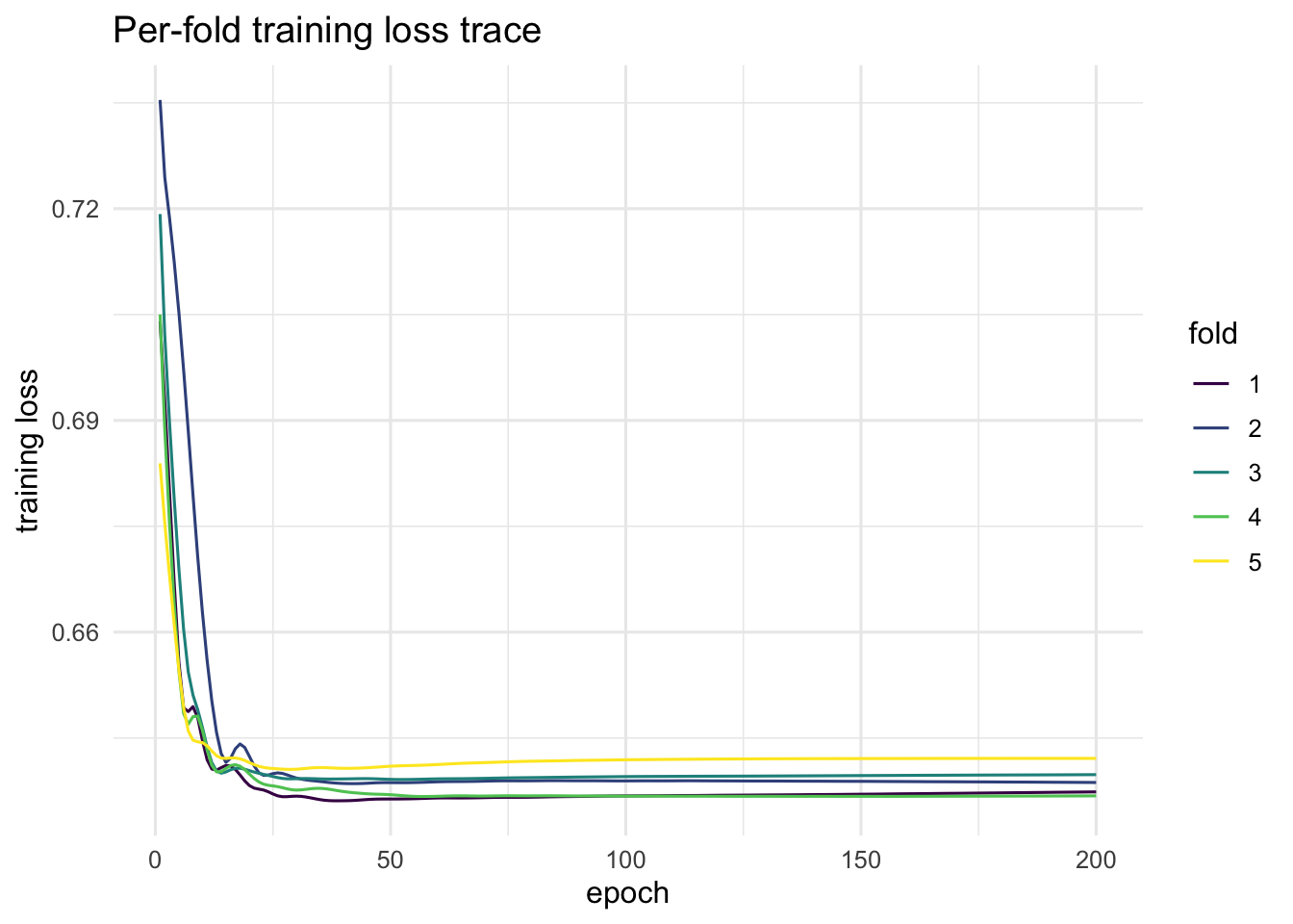
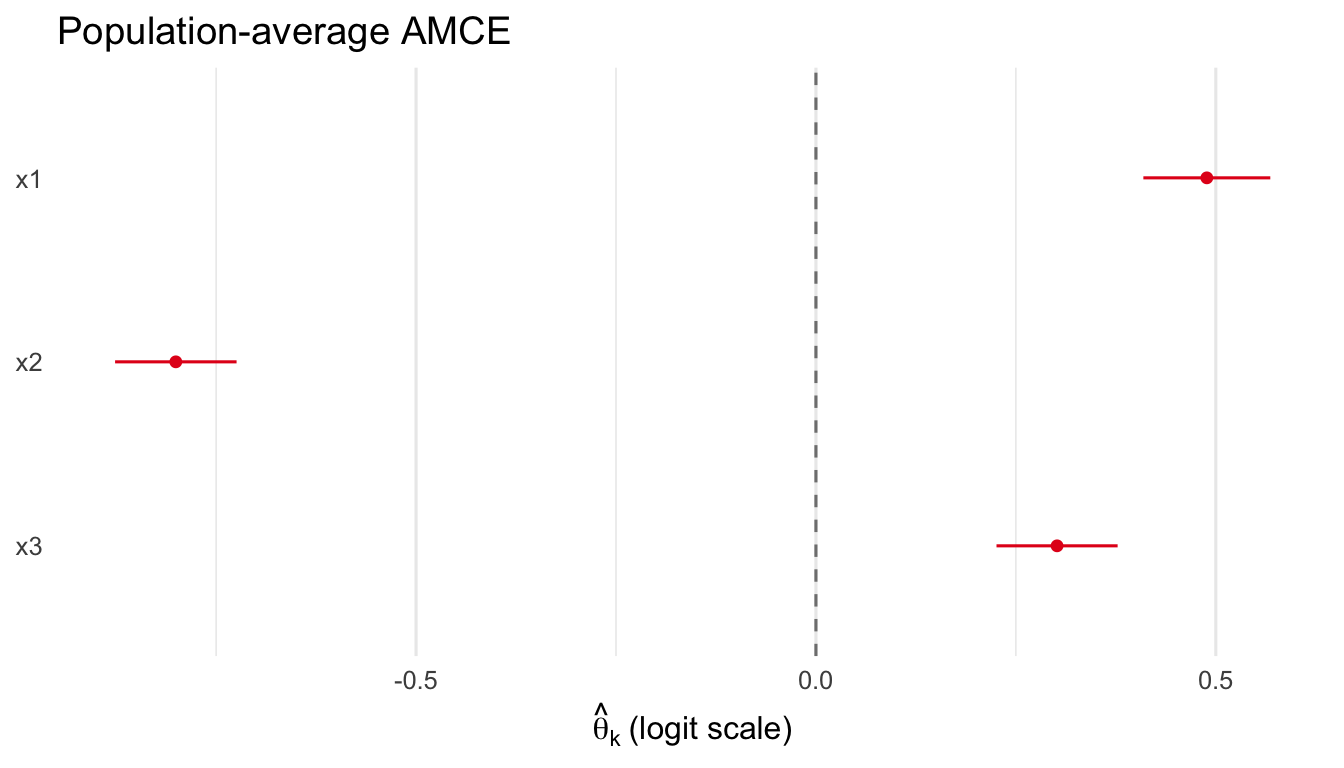
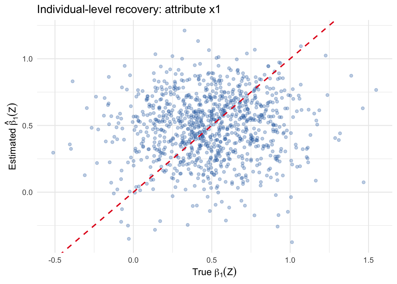
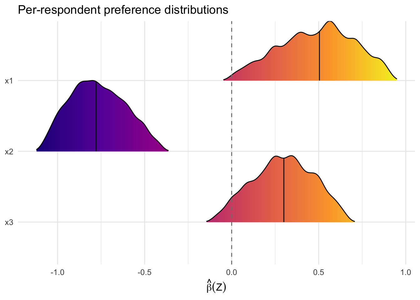
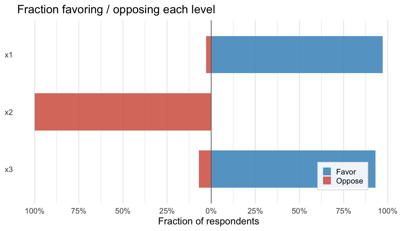
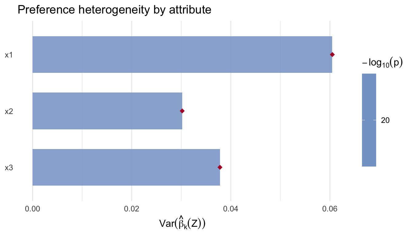
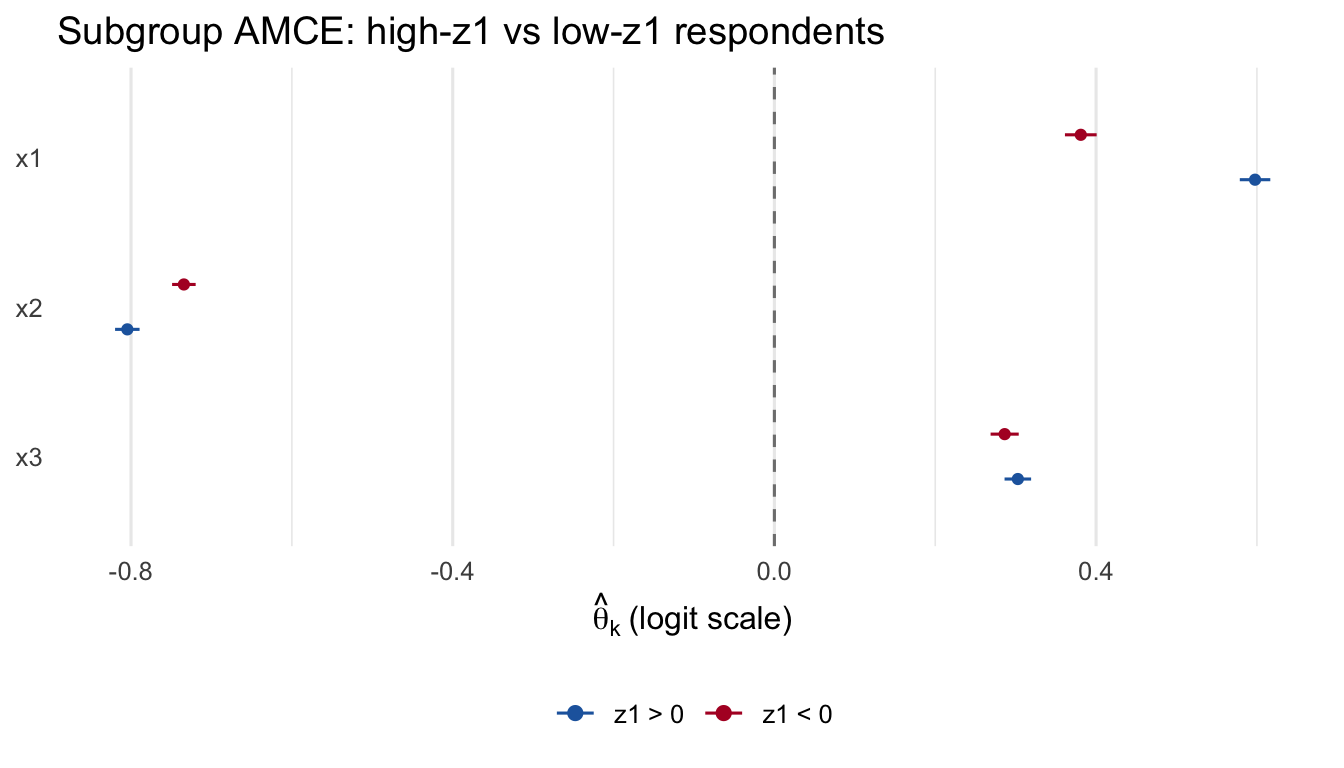
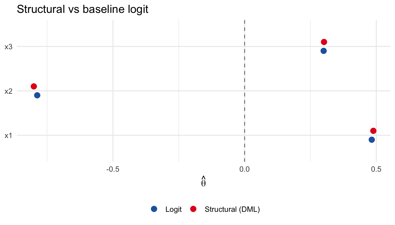
With these checks in hand, we proceed to real-data applications.