data(bs2013, package = "sconjoint")
dim(bs2013)
[1] 20000 13This dataset is included as a tutorial example to illustrate willingness-to-pay and compensating differential analysis with a numeric cost attribute. It is not one of the three main applications analyzed in the paper.
This chapter applies the structural estimator to a climate-treaty conjoint experiment whose design follows Bechtel and Scheve (2013). Respondents evaluate pairs of hypothetical international climate agreements varying on six attributes — including a numeric cost attribute (cost_usd) — and select the one they prefer. Because cost is numeric, this dataset is a natural showcase for willingness-to-pay (WTP) analysis via sc_wtp() and compensating differentials via sc_compensating().
data(bs2013, package = "sconjoint")
dim(bs2013)[1] 20000 13str(bs2013)'data.frame': 20000 obs. of 13 variables:
$ respondent : chr "122303373" "122303373" "122303373" "122303373" ...
$ task : int 1 1 2 2 3 3 4 4 1 1 ...
$ profile : int 1 2 1 2 1 2 1 2 1 2 ...
$ choice : int 0 1 0 1 1 0 1 0 0 1 ...
$ cost_usd : num 141 28 84 28 56 84 113 113 56 141 ...
$ distribution : Factor w/ 4 levels "Only rich pay",..: 2 3 2 1 3 4 2 4 3 3 ...
$ participation: Factor w/ 3 levels "20 countries",..: 3 3 2 2 1 3 3 2 1 2 ...
$ emissions : Factor w/ 3 levels "40% reduction",..: 1 2 3 1 2 2 3 1 2 2 ...
$ sanctions : Factor w/ 4 levels "No sanctions",..: 3 1 1 1 3 4 3 3 3 3 ...
$ monitoring : Factor w/ 4 levels "Your government",..: 3 4 4 2 4 4 3 1 4 4 ...
$ resp_female : num 1 1 1 1 1 1 1 1 1 1 ...
$ resp_age : num 57 57 57 57 57 57 57 57 52 52 ...
$ resp_ideo : num 2 2 2 2 2 2 2 2 7 7 ...Each respondent contributes four forced-choice tasks with two treaty profiles each (eight rows per respondent). The respondent-level moderators are resp_female (binary), resp_age (years), and resp_ideo (0–10 ideology).
fit_bs <- scfit(
  choice ~ cost_usd + distribution + participation + emissions +
           sanctions + monitoring |
           resp_female + resp_age + resp_ideo,
  data        = bs2013,
  respondent  = "respondent",
  task        = "task",
  profile     = "profile",
  K           = 5L,
  n_epochs    = 200L,
  seed        = 2024
)
summary(fit_bs)
sc_fit summary
Call: scfit(formula = choice ~ cost_usd + distribution + participation +
emissions + sanctions + monitoring | resp_female + resp_age +
resp_ideo, data = bs2013, respondent = "respondent", task = "task",
profile = "profile", K = 5L, n_epochs = 200L, seed = 2024)
2500 respondents | 10000 observations | K = 5 folds
hidden = 32-32-16 | epochs = 200 | seed = 2024 | device = cpu
Coefficients (DML, respondent-clustered SE):
estimate std_error z_value p_value
cost_usd -0.01500 0.0004967 -30.209 1.810e-200
distributionProp. current emissions 0.43510 0.0471880 9.221 2.953e-20
distributionProp. hist. emissions 0.46558 0.0464656 10.020 1.247e-23
distributionRich pay more, shared 0.36344 0.0445570 8.157 3.439e-16
participation80 countries 0.37278 0.0387545 9.619 6.640e-22
participation160 countries 0.65463 0.0419366 15.610 6.234e-55
emissions60% reduction 0.06353 0.0386110 1.645 9.989e-02
emissions80% reduction 0.13053 0.0396538 3.292 9.961e-04
sanctions$6/mo sanctions 0.10638 0.0466335 2.281 2.254e-02
sanctions$17/mo sanctions -0.16854 0.0457048 -3.688 2.263e-04
sanctions$23/mo sanctions -0.38426 0.0467863 -8.213 2.155e-16
monitoringIndependent commission 0.20502 0.0466952 4.391 1.131e-05
monitoringUnited Nations -0.07647 0.0483781 -1.581 1.140e-01
monitoringGreenpeace -0.18156 0.0489439 -3.709 2.077e-04
ci_lo ci_hi
cost_usd -0.01598 -0.01403
distributionProp. current emissions 0.34262 0.52759
distributionProp. hist. emissions 0.37451 0.55665
distributionRich pay more, shared 0.27611 0.45077
participation80 countries 0.29683 0.44874
participation160 countries 0.57243 0.73682
emissions60% reduction -0.01215 0.13921
emissions80% reduction 0.05281 0.20825
sanctions$6/mo sanctions 0.01498 0.19778
sanctions$17/mo sanctions -0.25812 -0.07896
sanctions$23/mo sanctions -0.47596 -0.29256
monitoringIndependent commission 0.11350 0.29654
monitoringUnited Nations -0.17129 0.01835
monitoringGreenpeace -0.27748 -0.08563
DML/iid SE ratio (mean): 1.052
Stage 2: map_c5 | mean(sigma_prior) = 250.1The Stage-2 MAP refinement runs by default for all scfit() calls. Set stage2 = "none" to recover v0.1 behavior. Note: this Bechtel- Scheve climate-policy example is not in the paper; it lives in the tutorial as a fourth showcase.
plot(fit_bs, "loss_trace")
plot_amce(fit_bs, groups = bs_groups, labels = bs_labels)
plot(fit_bs, "beta_ridgelines", groups = bs_groups, labels = bs_labels)
sc_importance(fit_bs)sc_quantity: importance
estimate: data.frame with 6 rows
attribute share se ci_lo ci_hi
cost_usd 0.72213 0.0067365 0.708930 0.73534
distribution 0.09259 0.0023163 0.088053 0.09713
participation 0.11203 0.0028572 0.106428 0.11763
emissions 0.01041 0.0004451 0.009542 0.01129
sanctions 0.03579 0.0009391 0.033947 0.03763
monitoring 0.02704 0.0008546 0.025369 0.02872plot_importance(fit_bs, labels = c(cost_usd = "Cost", distribution = "Distribution",
participation = "Participation", emissions = "Emissions",
sanctions = "Sanctions", monitoring = "Monitoring"))
sc_direction_intensity(fit_bs)sc_quantity_bivariate: direction_intensity
-- direction --
sc_quantity: direction
estimate: data.frame with 14 rows
dummy_name d se_d ci_lo_d ci_hi_d
cost_usd -0.5272 0.016998 -0.5605 -0.4939
distributionProp. current emissions 1.0000 0.000000 1.0000 1.0000
distributionProp. hist. emissions 1.0000 0.000000 1.0000 1.0000
distributionRich pay more, shared 1.0000 0.000000 1.0000 1.0000
participation80 countries 0.9992 0.000800 0.9976 1.0008
participation160 countries 1.0000 0.000000 1.0000 1.0000
emissions60% reduction 0.5136 0.017164 0.4800 0.5472
emissions80% reduction 0.6280 0.015567 0.5975 0.6585
sanctions$6/mo sanctions 0.9240 0.007649 0.9090 0.9390
sanctions$17/mo sanctions -0.9800 0.003981 -0.9878 -0.9722
... 4 more rows
-- intensity --
sc_quantity: intensity
estimate: data.frame with 14 rows
dummy_name u se_u ci_lo_u ci_hi_u
cost_usd 1.229e+03 4.010e+02 443.28658 2.015e+03
distributionProp. current emissions 4.203e-01 1.931e-03 0.41655 4.241e-01
distributionProp. hist. emissions 4.496e-01 2.495e-03 0.44472 4.545e-01
distributionRich pay more, shared 3.462e-01 1.181e-03 0.34392 3.485e-01
participation80 countries 3.422e-01 1.748e-03 0.33875 3.456e-01
participation160 countries 6.186e-01 2.414e-03 0.61383 6.233e-01
emissions60% reduction 7.703e-02 1.177e-03 0.07473 7.934e-02
emissions80% reduction 1.373e-01 1.954e-03 0.13344 1.411e-01
sanctions$6/mo sanctions 1.041e-01 1.015e-03 0.10206 1.060e-01
sanctions$17/mo sanctions 1.690e-01 1.386e-03 0.16632 1.718e-01
... 4 more rowssc_wtp() returns \(-\hat\beta_k / \hat\beta_{\text{cost}}\), the respondent-level cost the average voter would accept to gain feature \(k\), in the same units as cost_usd. Positive values mean the feature is desired enough that voters would pay for it.
## WTP for selected treaty features
sc_wtp(fit_bs, attr = "distributionRich pay more, shared", cost_attr = "cost_usd")
sc_quantity: wtp
estimate = 5.224 se = 1.348 95% CI = [2.581, 7.867]sc_wtp(fit_bs, attr = "emissions80% reduction", cost_attr = "cost_usd")sc_quantity: wtp
estimate = 0.381 se = 0.6485 95% CI = [-0.89, 1.652]sc_wtp(fit_bs, attr = "monitoringUnited Nations", cost_attr = "cost_usd")sc_quantity: wtp
estimate = -2.379 se = 0.7135 95% CI = [-3.778, -0.9808]How much cost would respondents accept to gain a preferred treaty feature? sc_compensating() computes the per-respondent ratio and reports the trimmed mean.
sc_compensating(fit_bs,
                benefit = "distributionRich pay more, shared",
                cost    = "cost_usd")
sc_quantity: compensating
estimate = 5.224 se = 1.348 95% CI = [2.581, 7.867]sc_compensating(fit_bs,
benefit = "emissions80% reduction",
cost = "cost_usd")sc_quantity: compensating
estimate = 0.381 se = 0.6485 95% CI = [-0.89, 1.652]frac_bs <- sc_fraction_preferring(fit_bs, threshold = 0)
frac_bs$estimate[, c("dummy_name", "frac_positive", "frac_negative")] dummy_name frac_positive frac_negative
1 cost_usd 0.2364 0.7636
2 distributionProp. current emissions 1.0000 0.0000
3 distributionProp. hist. emissions 1.0000 0.0000
4 distributionRich pay more, shared 1.0000 0.0000
5 participation80 countries 0.9996 0.0004
6 participation160 countries 1.0000 0.0000
7 emissions60% reduction 0.7568 0.2432
8 emissions80% reduction 0.8140 0.1860
9 sanctions$6/mo sanctions 0.9620 0.0380
10 sanctions$17/mo sanctions 0.0100 0.9900
11 sanctions$23/mo sanctions 0.0000 1.0000
12 monitoringIndependent commission 0.9916 0.0084
13 monitoringUnited Nations 0.2900 0.7100
14 monitoringGreenpeace 0.0348 0.9652plot_fraction(fit_bs, groups = bs_groups, labels = bs_labels)
Plot the per-attribute heterogeneity variance. Because the numeric cost_usd attribute is on a much larger scale than the 0/1 dummies, its MAP-shrunk per-respondent variance dominates a shared x-axis. We pass which_beta = "dnn" (read the well-scaled Stage-1 view) and facet_scales = "free" (each attribute group gets its own x range).
plot_hetero(fit_bs, groups = bs_groups, labels = bs_labels,
            which_beta = "dnn", facet_scales = "free")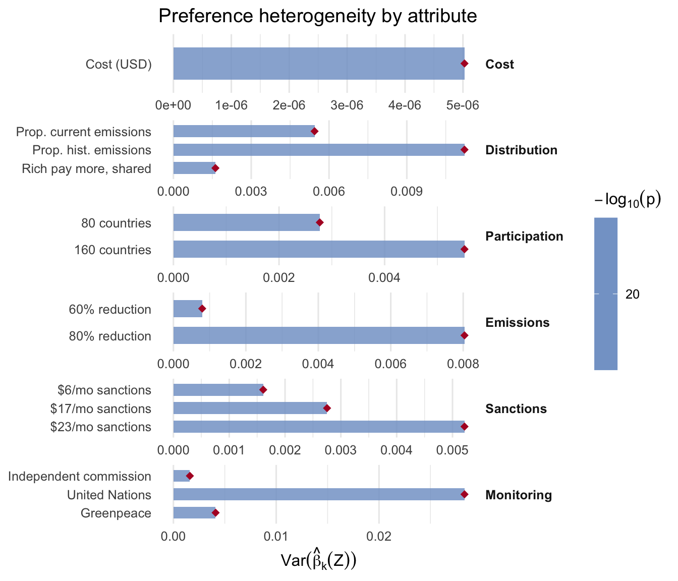
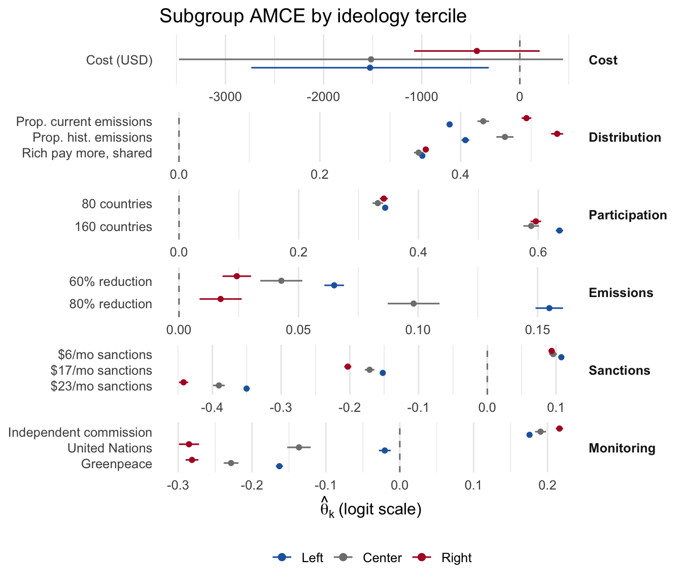
ideo_col <- fit_bs$Z[, "resp_ideo"]
ideo_cuts <- quantile(ideo_col, probs = c(1/3, 2/3))
plot_subgroup(
  fit_bs,
  subgroup = list(Left   = ideo_col <= ideo_cuts[1],
                  Center = ideo_col > ideo_cuts[1] & ideo_col <= ideo_cuts[2],
                  Right  = ideo_col > ideo_cuts[2]),
  groups = bs_groups, labels = bs_labels,
  title = "Subgroup AMCE by ideology tercile"
)
The climate application is a teaching example rather than one of the paper’s three applications, included to show the workflow on a design with a numeric cost attribute: