This chapter walks through a complete sconjoint analysis of a candidate-choice conjoint experiment whose design follows Saha and Weeks (2022). Respondents evaluate pairs of hypothetical political candidates varying on five attributes and select one. The structural decomposition into direction and intensity lets us ask whether a near-zero AMCE for candidate gender masks genuine heterogeneity — half the sample preferring women, half preferring men.
3.1 Data preparation
Load the bundled Saha-Weeks subset and inspect its structure.
The data are in long format: one row per respondent–task–profile. Each respondent contributes three forced-choice tasks; within a task two candidate profiles are presented and exactly one is chosen (choice == 1).
For consistency with the paper, we re-level cand_gender so that Female is the reference and Male is the non-reference dummy. The paper reports the Male-relative-to-Female coefficient throughout.
The respondent-level moderators available in \(\mathbf Z\) are resp_female (binary), age (standardized), and pid (3-level partisanship index). The formula interface puts conjoint attributes to the left of | and moderators to the right:
choice ~ agenda + talent + children + cand_gender + prior_office |
         resp_female + age + pid
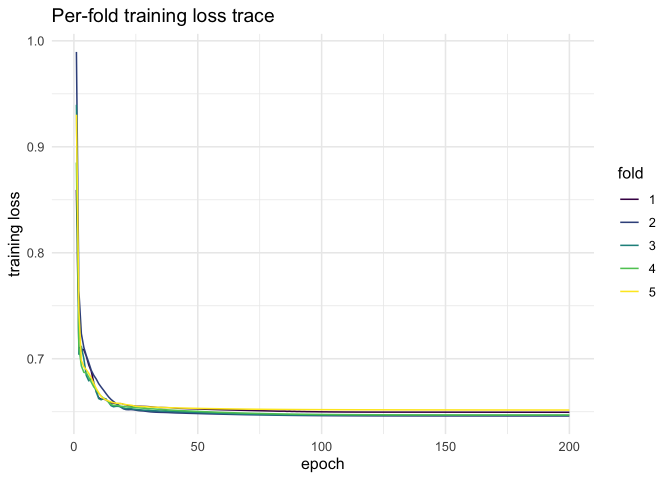
3.2 Fitting
We fit a moderate configuration (K = 5 folds, 200 Adam epochs) that balances render speed against paper-quality estimates. A production run would use K = 10 and n_epochs >= 1000. The loss trace below shows the per-fold training curves; with K = 5 cross-fitting the loss has largely plateaued by epoch 150-200.
As of v0.2, scfit() runs an empirical-Bayes MAP refinement (paper EnsC5) on top of the Stage-1 DNN by default (stage2 = "map_c5"). The summary above reports this as Stage 2: map_c5. DML point estimates and clustered standard errors are unchanged from v0.1 — they continue to use the Stage-1 single-DNN prediction (now stored on fit_sw$beta_hat_dnn). The refined betas (fit_sw$beta_hat) feed every distributional and individual-level quantity below. Set stage2 = "none" to recover v0.1 behavior, or stage2 = "mixed_logit" for the BLUP alternative from paper §A.4.
3.3 Population-average estimates
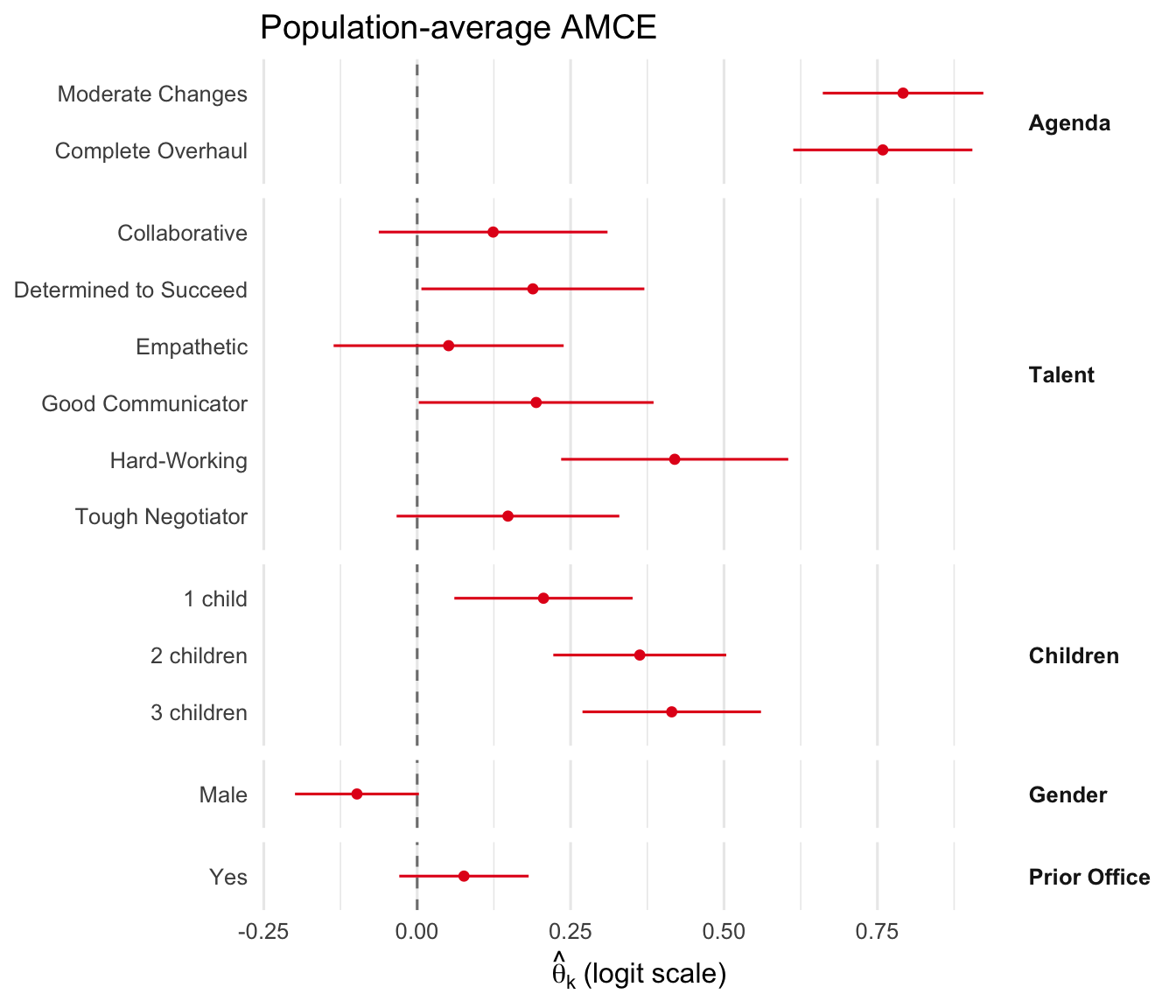
The DML point estimates \(\hat\theta_k\) on the logit scale. Inspect numerically, then visualize as a coefficient plot grouped by attribute.
plot_amce(fit_sw, groups = sw_groups, labels = sw_labels)
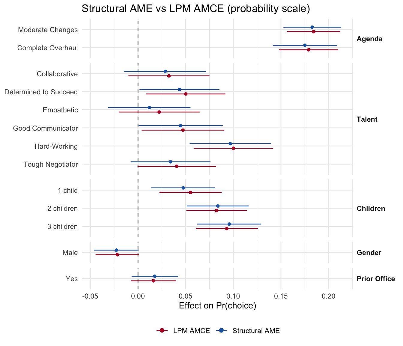
3.3.1 Structural AME vs reduced-form AMCE (paper Figure 1.B)
The paper notes that the structural model’s average marginal effect (AME) on the probability scale nearly coincides with the standard linear-probability-model AMCE — confirming that the structural estimator nests reduced-form AMCE analysis. Below we compute both and overlay them as point-ranges on the probability scale.
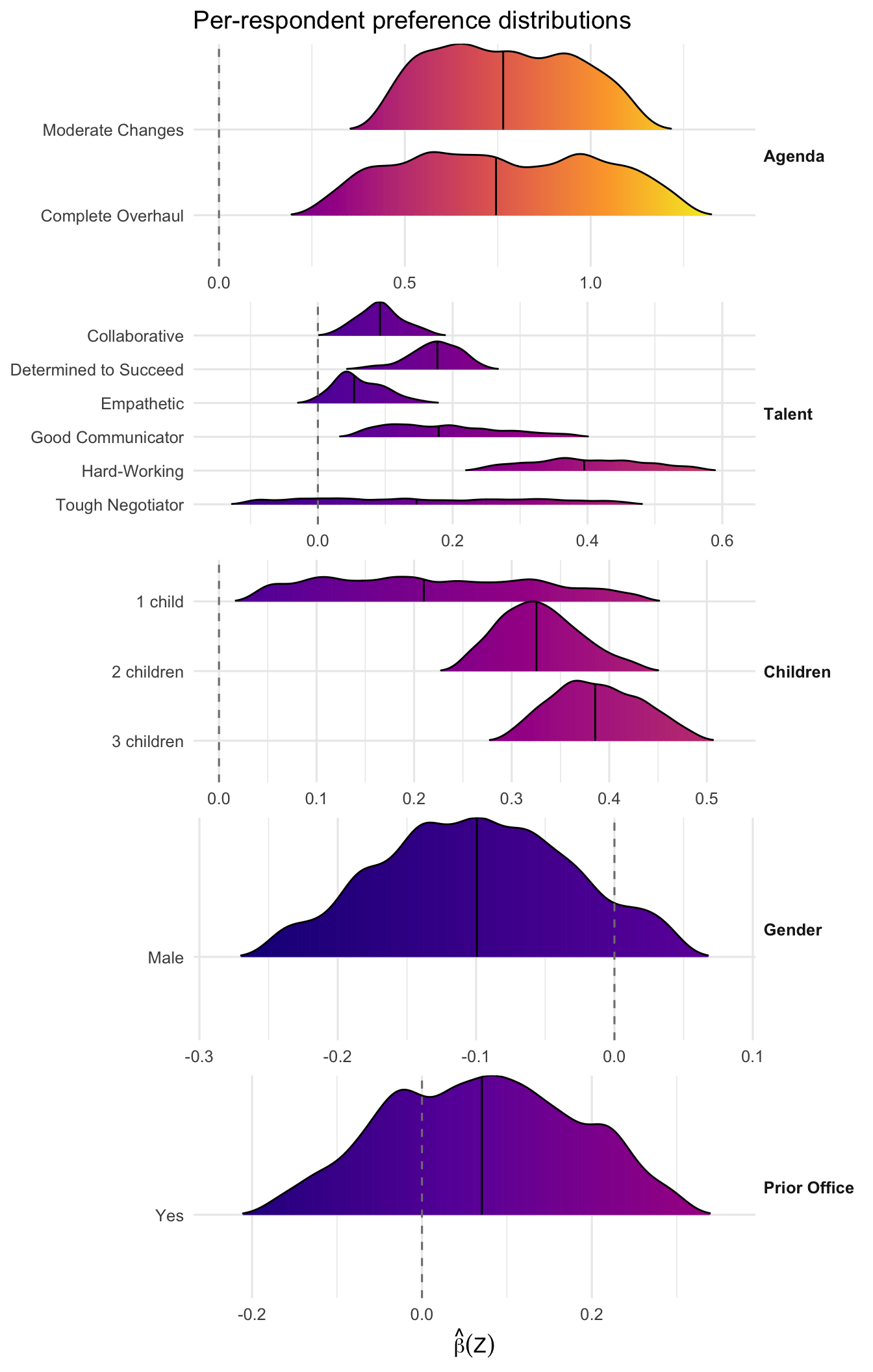
Ridgeline densities show the distribution of \(\hat\beta_k(\mathbf Z_i)\) per dummy across respondents. The vertical dashed line is at zero; the solid line in each density is the median.
plot(fit_sw, "beta_ridgelines", groups = sw_groups, labels = sw_labels)
3.5 Structural quantities
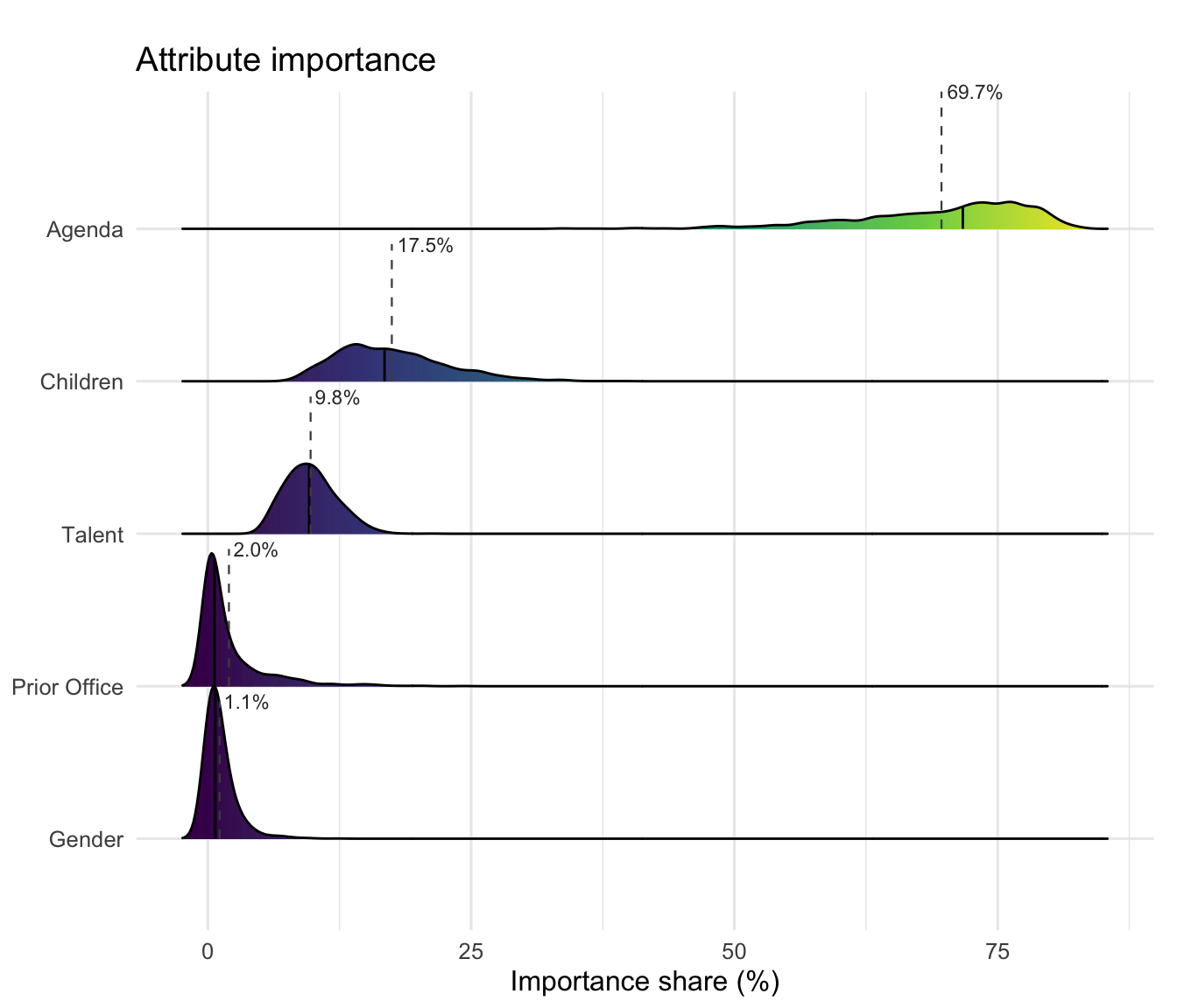
3.5.1 Attribute importance
Variance-decomposition share of utility carried by each attribute group, averaged across respondents. The “importance” answers: which attribute moves the choice the most?
Policy agenda dominates the decision variance for the median voter, ranking well above the other attributes. Read the exact shares off the plot above rather than quoting a fixed fraction — on the bundled data they reflect the reduced moderator set (see the note in the overview).
3.5.2 Direction and intensity
For each dummy, decompose preference into a direction (the sign of \(\hat\beta_{ik}\)) and an intensity (its magnitude). Near-zero average effects can hide either consensus (everyone close to zero) or polarization (large opposing intensities cancelling).
For the Empathetic attribute, the near-zero average masks an almost perfectly polarized electorate: approximately half favor empathetic candidates while the other half oppose them.
3.5.3 Fraction preferring
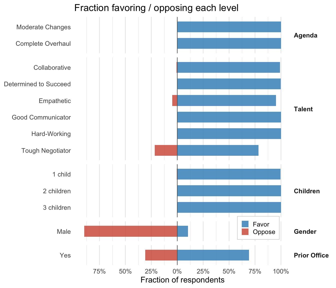
What share of respondents have a positive coefficient on each dummy? This is the direction-only summary — ignores intensity.
plot_fraction(fit_sw, groups = sw_groups, labels = sw_labels)
The paper’s directional finding for gender: the population-average AMCE for Male is near zero, but the individual-level fractions reveal that a clear majority of respondents have \(\hat\beta_{\text{Male}} < 0\), i.e. prefer Female candidates. The fraction-preferring panel above makes this visible per dummy. (Read the exact share off the rendered table rather than quoting a fixed number — it depends on the training configuration and, on the bundled data, on the reduced moderator set.)
3.5.4 Marginal rate of substitution
The respondent-averaged trimmed ratio \(\hat\beta_j / \hat\beta_k\) between two dummies, with respondent-clustered SE. Trimming at \(\{0.01, 0.99\}\) guards the unbounded ratio when the denominator is near zero.
sc_mrs(fit_sw, numerator =1L, denominator =2L)
sc_quantity: mrs
  estimate = 1.102   se = 0.01019   95% CI = [1.082, 1.122]
TipLarge trimmed mean?
The ratio \(\hat\beta_j / \hat\beta_k\) is unbounded when the denominator is near zero. Inspect the ridgelines above to confirm the denominator column is well-separated from zero.
3.5.5 Counterfactual choice probability
Predicted choice probability for a specific head-to-head profile pair, averaged across respondents. Each profile is a named list of attribute levels; unmentioned attributes default to the reference level.
sc_counterfactual( fit_sw,## Profile A: a Female Hard-Working candidate proposing a Complete## Overhaul, against B: a Male Assertive candidate proposing the## minimal change. Female is the reference level so it does not## appear in the dummy contrast; Male contributes +beta_Male to A's## utility (negative in this design).A =list(agenda ="Complete Overhaul", talent ="Hard-Working",children ="2 children", cand_gender ="Female",prior_office ="Yes"),B =list(agenda ="Very Few Changes", talent ="Assertive",children ="No children", cand_gender ="Male",prior_office ="No"))
sc_quantity: counterfactual
  estimate = 0.8345   se = 0.001346   95% CI = [0.8319, 0.8371]
3.5.6 Optimal profile
The single profile that maximizes the population-average utility (greedy attribute-by-attribute selection over the discrete attribute levels).
sc_optimal_profile(fit_sw)
sc_quantity: optimal_profile
  estimate = 0.8324   se = 0.001054   95% CI = [0.8304, 0.8345]
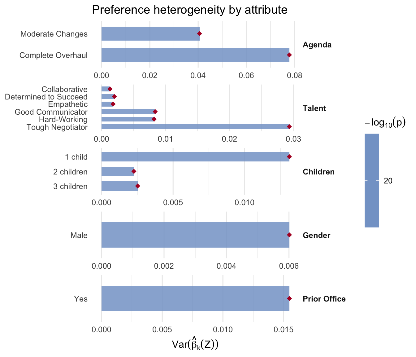
3.5.7 Heterogeneity test
For each dummy, the one-sided test that \(\mathrm{Var}(\beta_k(Z)) > 0\) exceeds zero. Useful for screening which attributes genuinely vary across respondents.
plot_hetero(fit_sw, groups = sw_groups, labels = sw_labels)
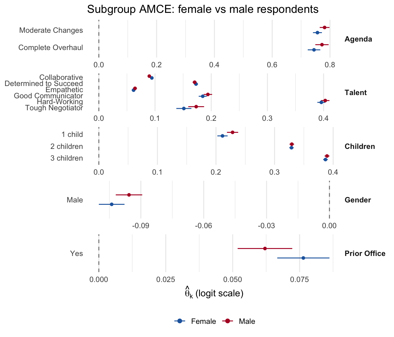
3.5.8 Subgroup analysis
Re-average the respondent-level betas over a subset of respondents, then compare across subsets. Below: compare the per-attribute means for female vs male respondents on the gender attribute.
New in v0.2.1: sc_design_diagnostic() estimates per-coefficient \(\hat R^2_{Z,k}\) from the MAP posterior and reports which recovery tiers the design supports (mean / distributional / individual / ratio) per the paper §6 heuristics. On the Saha-Weeks design (T ≈ 3, modest covariate set), expect mean-only support; the talent attributes are well-pinned by Z, while gender and prior-office rely most on T.
sc_design_diagnostic(fit_sw)
sc_design_diagnostic --- recovery-tier hint
[experimental: estimator over-estimates R^2_Z when Z is
 uninformative (validation bias +0.4 at true R^2_Z = 0.10).
 Use for relative comparisons across coefficients; do not
 treat tier hints as a pass/fail gate.  See ?sc_design_diagnostic.]
Stage 2: map_c5
Respondents: 1191 | Tasks: 3573 | T_mean: 3 | mean R^2_Z: 0.361

Recovery tiers:
  [YES] mean & aggregate        (any reasonable design)
  [NO]  distributional          (T >= 5 and R^2_Z >= 0.35)
  [NO]  individual-level        (T >= 8 and R^2_Z >= 0.55)
  [NO]  ratio (MRS / WTP)       (T >= 10 and R^2_Z >= 0.55 and N >= 5000)

Top coefficients by R^2_Z (best-pinned by Z):
  talentTough Negotiator          0.936
  talentGood Communicator         0.807
  talentHard-Working              0.805
  talentDetermined to Succeed     0.501
  talentEmpathetic                0.475
Bottom coefficients (rely most on T for recovery):
  children1 child                 0.183
  children3 children              0.0433
  prior_officeYes                 0.0344
  children2 children              0.0235
  cand_genderMale                 0.00671
3.5.11 Validating against the homogeneous-logit AMCE
The paper’s Appendix D shows that the structural model nests the standard reduced-form AMCE: the DML population-average parameter \(\theta_k = \mathbb{E}[\beta_k(Z)]\) equals the pooled homogeneous-logit coefficient on attribute \(k\) when the logit specification holds. The sc_validate_amce() export turns this into a one-line sanity check.
In a full paper-quality fit (K = 10, n_epochs >= 1000) the correlation across attribute levels is very high (close to 1). Any material drop is a sign of either insufficient training or a genuinely non-logit data-generating process.
3.5.12 Comparing the Stage-2 view to the raw DNN view
Every sc_* quantity now accepts a which_beta argument with default "hybrid" (Stage-2 refined). Passing "dnn" reads the unrefined Stage-1 DNN mean, which lives in fit_sw$beta_hat_dnn.
The Stage-2 refinement typically shifts the more polarized columns (e.g. cand_genderMale, talentEmpathetic) toward smaller fractions and the consensus columns (talentHard-Working, agendaModerate Changes) toward 100% — this is the within-respondent shrinkage at work.