This chapter applies the structural estimator to a tax-plan conjoint experiment from Ballard-Rosa, Martin, and Scheve (2017). Respondents evaluate pairs of hypothetical income tax plans varying on six marginal tax rates (one per income bracket) plus a revenue impact indicator, and select the plan they prefer.
What makes this dataset unique among the bundled examples is that every attribute is numeric (continuous). There are no factor attributes — the six bracket rates are percentages and the revenue score is a centered integer scale. This showcases how sconjoint handles all-numeric attribute designs.
Each respondent contributes eight forced-choice tasks with two tax-plan profiles each (16 rows per respondent). The respondent-level moderators include demographics (age, gender, education, race, income), partisanship (resp_pid7, 1–7), and economic attitudes (inequality aversion, work-vs-luck beliefs, taxes-harm beliefs, hard-work beliefs, economic knowledge, employment status) — 12 moderators in total.
5.2 Fitting the structural model
Every attribute here is continuous, with the tax rates encoded as percentage points (0–50). The paper handles this with the varref Stage-2 prior and a low variance floor (varref_floor = 1e-3) on the raw rates, rather than the default score-based map_c5 prior. We follow the paper’s recipe here. Coefficients are in “logit utility per percentage point” units.
NoteWhy stage2 = "varref" for continuous attributes?
The default map_c5 Stage-2 prior is calibrated assuming \(\mathrm{Var}(\Delta X_k) \approx 1\) (true for factor dummies under typical randomization). BR’s tax rates span 0–50 percentage points, so the score-based prior becomes loose and the MAP solver leaves per-respondent estimates with extreme tails. The paper instead uses the varref prior — \(0.5\cdot\mathrm{Var}_i(\hat\beta_{\text{ens},i,k})\), floored at varref_floor — on the raw rates. The low floor matters: the prior 0.01 default over-shrinks continuous coefficients and badly degrades recovery of individual progressivity, so continuous designs use varref_floor = 1e-3 (the paper’s setting). An alternative is normalize_deltaX = TRUE with the default map_c5 prior, which standardizes \(\Delta X\) internally; see the Advanced options chapter. For factor-dummy designs (SW, GS) neither is needed.
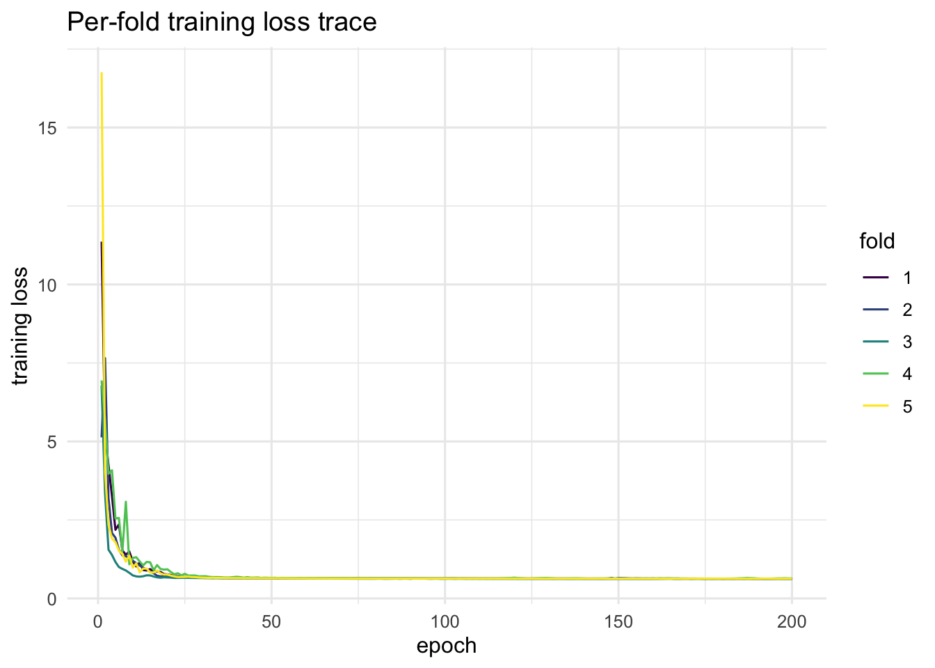
plot(fit_br, "loss_trace")
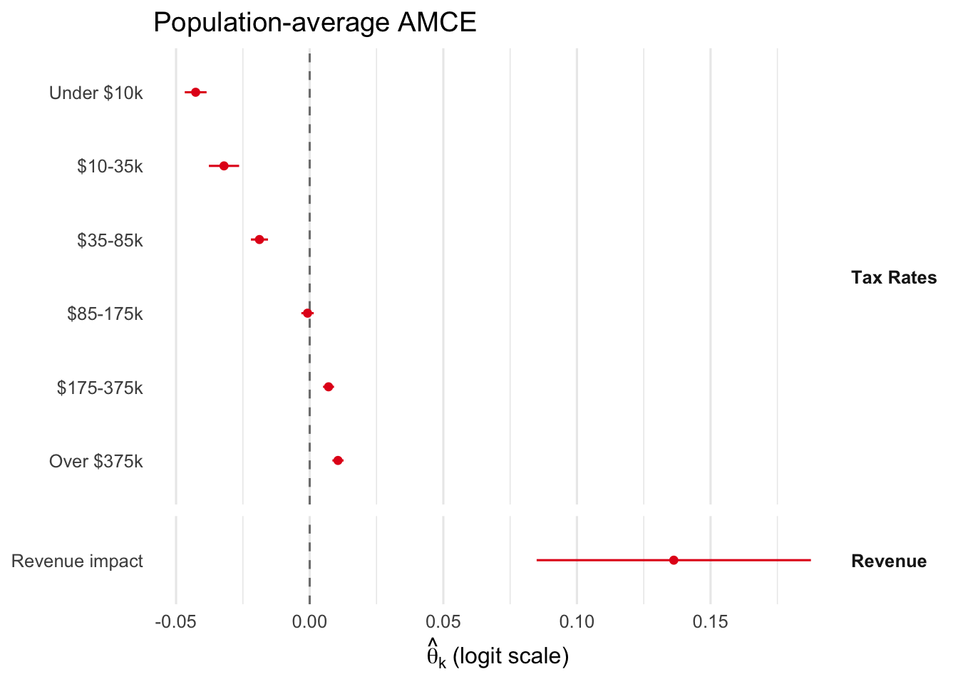
5.3 Population-average estimates
DML coefficients per attribute, on the logit scale, with respondent- clustered SEs. With numeric attributes the coefficient is “logit utility per unit of the attribute” (per percentage-point of the rate, or per unit of the centered revenue indicator).
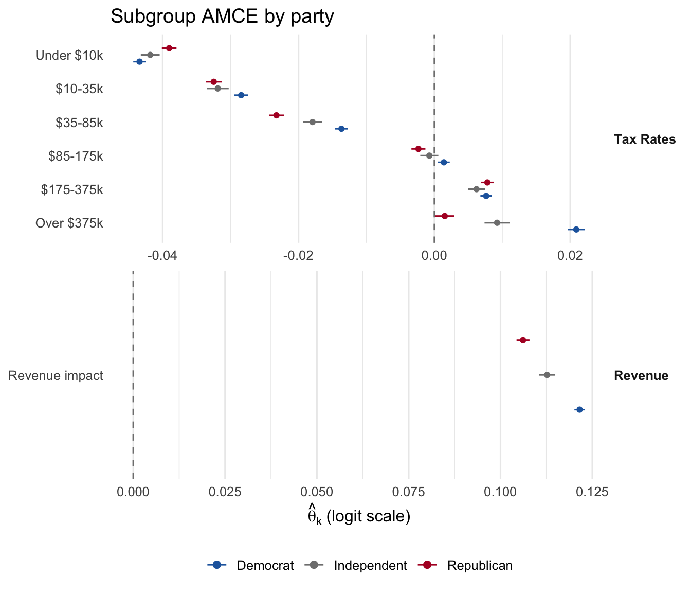
plot_amce(fit_br, groups = br_groups, labels = br_labels)
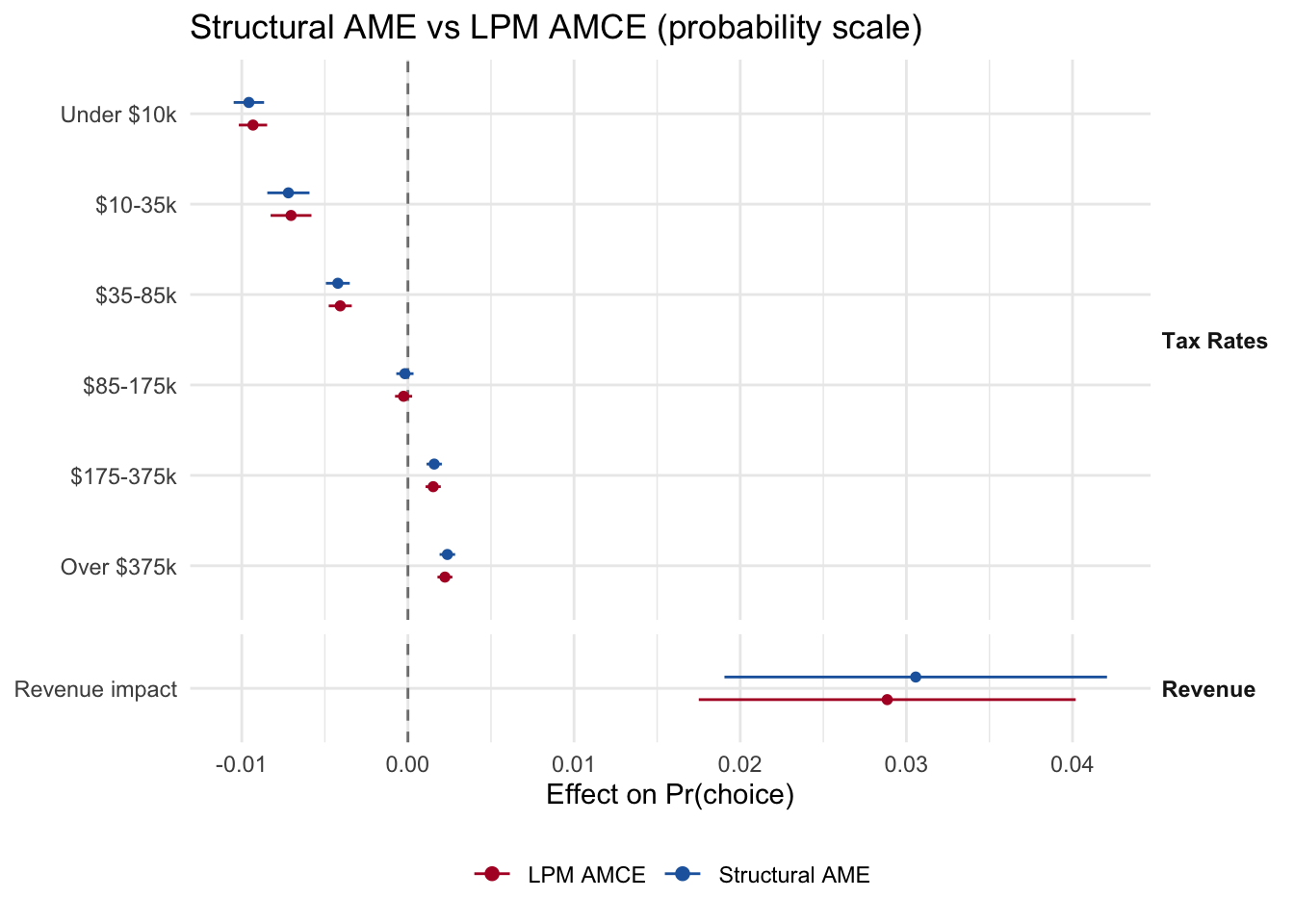
5.3.1 Structural AME vs reduced-form AMCE
For continuous attributes the AME is “average effect on Pr(choice) per unit of the attribute”. Overlay the structural and LPM versions on the probability scale.
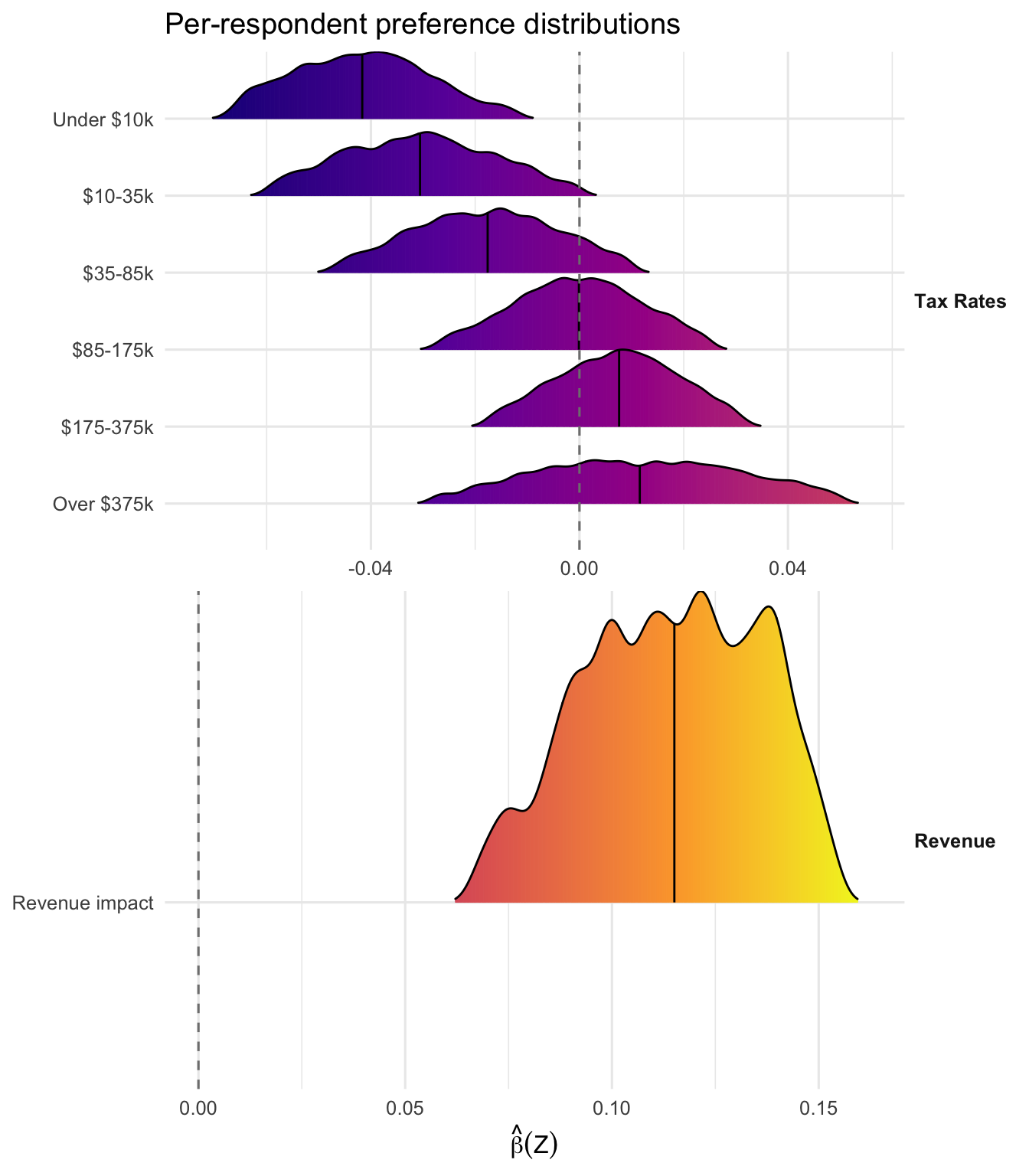
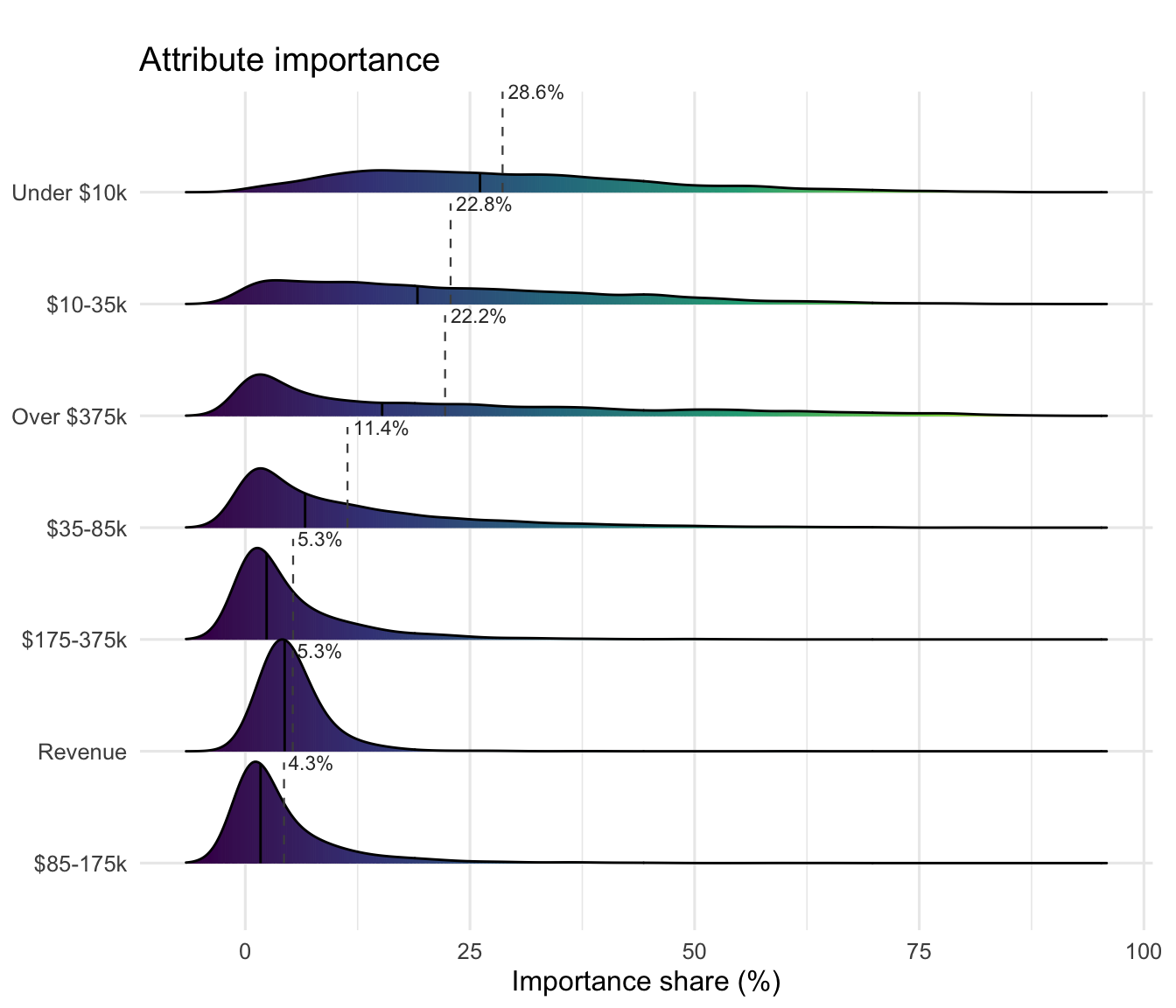
Ridgeline densities of \(\hat\beta_k(\mathbf Z_i)\) per attribute across respondents. With normalize_deltaX = TRUE the MAP refinement is properly scaled — the hybrid view shows clean per-respondent distributions for every bracket.
plot(fit_br, "beta_ridgelines", groups = br_groups, labels = br_labels)
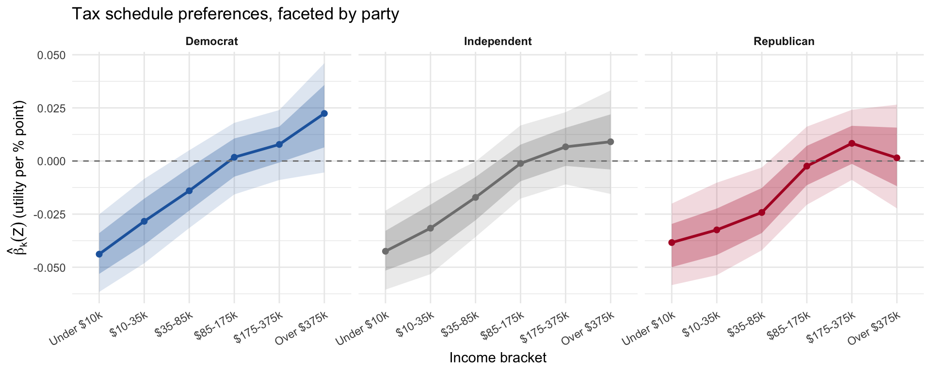
This plot is unique to the tax-plan conjoint. It extracts the six bracket coefficients \(\hat\beta_k(\mathbf Z_i)\) and shows the respondent-level preferred-rate schedule in three panels (one per party). The dark ribbon is the interquartile range across respondents within each party; the light ribbon is the 10th–90th percentile range.
Nearly all respondents exhibit progressive tax preferences (a positive slope from low to high brackets), and progressivity remains the majority pattern even among Republicans. The partisan gap is real but modest — Democrats’ mean slope is somewhat steeper than Republicans’. (These shares are computed on the bundled data; read the exact values off the rendered output rather than quoting fixed numbers.)
Under correct logit specification, the DML \(\hat\theta\) on each tax bracket matches the pooled logit’s coefficient on the same bracket exactly. The pooled correlation is the cleanest summary that the structural model loses nothing the AMCE delivers.