4  Example: Democratic Norms

This chapter applies the structural estimator to a candidate-choice conjoint whose design follows Graham and Svolik (2020). Respondents choose between pairs of hypothetical U.S. candidates; one attribute captures the candidate’s willingness to engage in undemocratic behavior (ignoring a court ruling, restricting the opposition press, or banning an opposition rally). The original study asks how much voters penalize co-partisan candidates for violating democratic norms, and whether strong partisanship leads to tolerance of such violations.

The structural model adds value here because it decomposes the population-average penalty for undemocratic behavior into direction and intensity, and traces the heterogeneity back to respondent-level partisanship — without re-estimating on subsets.

4.1 Data preparation

Load the Graham-Svolik subset and inspect its structure. Each respondent contributes about 13 forced-choice tasks against pairs of hypothetical candidates.

data(gs2020, package = "sconjoint")
dim(gs2020)
[1] 41314    23
head(gs2020, 4)
  respondent task profile choice copartisan p1 p2     dem_code cand_sex
1          1    1       1      0        Not  2  1    u_gerry10   Female
2          1    1       2      1        Not  4  3   g_schedule     Male
3          1    2       1      1        Not  4  3   g_schedule     Male
4          1    2       2      0        Not  1  4 g_boardElect   Female
  cand_race             cand_pro resp_ideo resp_pid resp_trump resp_age
1     White               Lawyer         6        3          4       71
2     White  Legislative staffer         6        3          4       71
3     White               Lawyer         6        3          4       71
4     Black Small business owner         6        3          4       71
  resp_female resp_race_black resp_race_asian resp_race_other resp_educ
1           0               0               0               0         2
2           0               0               0               0         2
3           0               0               0               0         2
4           0               0               0               0         2
  resp_income resp_auth resp_knowledge
1           8         1              7
2           8         1              7
3           8         1              7
4           8         1              7
str(gs2020)
'data.frame':   41314 obs. of  23 variables:
 $ respondent     : chr  "1" "1" "1" "1" ...
 $ task           : int  1 1 2 2 3 3 4 4 5 5 ...
 $ profile        : int  1 2 1 2 1 2 1 2 1 2 ...
 $ choice         : int  0 1 1 0 0 1 1 0 0 1 ...
 $ copartisan     : Factor w/ 2 levels "Not","Co-partisan": 1 1 1 1 1 1 2 1 1 2 ...
 $ p1             : num  2 4 4 1 4 3 1 3 1 4 ...
 $ p2             : num  1 3 3 4 3 4 4 2 3 1 ...
 $ dem_code       : Factor w/ 16 levels "g_boardElect",..: 12 7 7 1 7 6 14 4 10 6 ...
 $ cand_sex       : Factor w/ 2 levels "Male","Female": 2 1 1 2 2 2 1 2 1 2 ...
 $ cand_race      : Factor w/ 4 levels "White","Black",..: 1 1 1 2 1 1 1 1 1 1 ...
 $ cand_pro       : Factor w/ 9 levels "Business executive",..: 3 4 3 8 3 9 2 3 5 2 ...
 $ resp_ideo      : num  6 6 6 6 6 6 6 6 6 6 ...
 $ resp_pid       : num  3 3 3 3 3 3 3 3 3 3 ...
 $ resp_trump     : num  4 4 4 4 4 4 4 4 4 4 ...
 $ resp_age       : num  71 71 71 71 71 71 71 71 71 71 ...
 $ resp_female    : num  0 0 0 0 0 0 0 0 0 0 ...
 $ resp_race_black: num  0 0 0 0 0 0 0 0 0 0 ...
 $ resp_race_asian: num  0 0 0 0 0 0 0 0 0 0 ...
 $ resp_race_other: num  0 0 0 0 0 0 0 0 0 0 ...
 $ resp_educ      : num  2 2 2 2 2 2 2 2 2 2 ...
 $ resp_income    : int  8 8 8 8 8 8 8 8 8 8 ...
 $ resp_auth      : num  1 1 1 1 1 1 1 1 1 1 ...
 $ resp_knowledge : num  7 7 7 7 7 7 7 7 7 7 ...

Each respondent sees up to 13 matchups with two candidate profiles each. The respondent-level moderators include ideology (resp_ideo, 1–7), party identification (resp_pid, -3 to 3), Trump approval (resp_trump, 1–4), demographics (age, gender, race, education, income), and dispositional measures (authoritarianism, political knowledge) — 12 moderators in total. This is a reduced set relative to the paper (see the overview), so the numbers below are illustrative.

The dem_code attribute has 16 levels in three families: good-governance (g_*, 7 levels), undemocratic actions (u_*, 7 levels), and valence violations (v_*, 2 levels). The raw choice rates make the families crystal clear:

agg <- aggregate(choice ~ dem_code, data = gs2020, FUN = mean)
agg[order(-agg$choice), ]
            dem_code    choice
2        g_committee 0.5865261
1       g_boardElect 0.5752534
4        g_procedure 0.5717989
5         g_progEval 0.5703166
7         g_schedule 0.5635560
3  g_officestructure 0.5622132
6           g_record 0.5593487
11          u_gerry2 0.4135764
10        u_execRule 0.4030227
8       u_banProtest 0.3922062
12         u_gerry10 0.3840809
9            u_court 0.3687854
14       u_limitVote 0.3659924
13     u_journalists 0.3469773
15          v_affair 0.3419558
16             v_tax 0.2939698

Every g_* item is chosen at rate \(> 0.55\); every u_* item at rate \(< 0.42\); every v_* item at rate \(< 0.35\). The labels are correct. But the default factor reference is g_boardElect (alphabetically first), so when we fit the model with default contrasts, the g_* coefficients are estimated relative to another good-governance item, which makes the within-g_ comparisons noisy and a few of them slightly negative.

To get a more interpretable plot that lines up with the paper’s “voters favor good governance” finding, we re-level dem_code so that the reference is the mildest undemocratic action, u_gerry2 (slight gerrymandering). With this baseline, every g_* item shows a clearly positive coefficient (good-governance preferred over mild undemocratic behavior), other u_* items are near-zero or negative (worse than mild gerry), and v_* valence items are strongly negative.

gs2020$dem_code <- stats::relevel(factor(gs2020$dem_code),
                                  ref = "u_gerry2")
levels(gs2020$dem_code)[1]   # confirm new reference
[1] "u_gerry2"

4.2 Fitting the structural model

fit_gs <- scfit(
  choice ~ copartisan + p1 + p2 + dem_code + cand_sex + cand_race + cand_pro |
           resp_ideo + resp_pid + resp_trump + resp_age + resp_female +
           resp_race_black + resp_race_asian + resp_race_other +
           resp_educ + resp_income + resp_auth + resp_knowledge,
  data        = gs2020,
  respondent  = "respondent",
  task        = "task",
  profile     = "profile",
  K           = 5L,
  n_epochs    = 200L,
  seed        = 2024
)
summary(fit_gs)
sc_fit summary
Call: scfit(formula = choice ~ copartisan + p1 + p2 + dem_code + cand_sex + 
    cand_race + cand_pro | resp_ideo + resp_pid + resp_trump + 
    resp_age + resp_female + resp_race_black + resp_race_asian + 
    resp_race_other + resp_educ + resp_income + resp_auth + resp_knowledge, 
    data = gs2020, respondent = "respondent", task = "task", 
    profile = "profile", K = 5L, n_epochs = 200L, seed = 2024)

1605 respondents | 20657 observations | K = 5 folds
hidden = 32-32-16 | epochs = 200 | seed = 2024 | device = cpu

Coefficients (DML, respondent-clustered SE):
                              estimate std_error   z_value   p_value    ci_lo
copartisanCo-partisan         0.640227   0.03072  20.84229 1.791e-96  0.58002
p1                           -0.205825   0.01304 -15.78296 4.076e-56 -0.23139
p2                           -0.111760   0.01433  -7.80012 6.185e-15 -0.13984
dem_codeg_boardElect          0.474505   0.05857   8.10118 5.443e-16  0.35971
dem_codeg_committee           0.522124   0.06056   8.62213 6.572e-18  0.40344
dem_codeg_officestructure     0.430561   0.06116   7.04015 1.920e-12  0.31069
dem_codeg_procedure           0.435148   0.05977   7.28069 3.321e-13  0.31801
dem_codeg_progEval            0.455910   0.05897   7.73105 1.067e-14  0.34033
dem_codeg_record              0.388076   0.05972   6.49813 8.133e-11  0.27102
dem_codeg_schedule            0.422712   0.05936   7.12061 1.075e-12  0.30636
dem_codeu_banProtest         -0.063768   0.07475  -0.85309 3.936e-01 -0.21028
dem_codeu_court              -0.196589   0.07606  -2.58467 9.747e-03 -0.34566
dem_codeu_execRule           -0.036036   0.07403  -0.48679 6.264e-01 -0.18113
dem_codeu_gerry10            -0.138358   0.07153  -1.93416 5.309e-02 -0.27856
dem_codeu_journalists        -0.323482   0.07580  -4.26780 1.974e-05 -0.47204
dem_codeu_limitVote          -0.204337   0.07602  -2.68812 7.186e-03 -0.35332
dem_codev_affair             -0.357735   0.07400  -4.83439 1.336e-06 -0.50277
dem_codev_tax                -0.581193   0.07657  -7.59064 3.183e-14 -0.73126
cand_sexFemale                0.041219   0.02347   1.75631 7.904e-02 -0.00478
cand_raceBlack               -0.002324   0.03320  -0.06999 9.442e-01 -0.06739
cand_raceHispanic            -0.085516   0.03251  -2.63026 8.532e-03 -0.14924
cand_raceAsian               -0.101415   0.05084  -1.99467 4.608e-02 -0.20107
cand_proFarmer                0.050921   0.04579   1.11196 2.662e-01 -0.03883
cand_proLawyer                0.039711   0.03737   1.06272 2.879e-01 -0.03353
cand_proLegislative staffer   0.062858   0.04319   1.45529 1.456e-01 -0.02180
cand_proPolice officer        0.072957   0.04545   1.60527 1.084e-01 -0.01612
cand_proServed in the army    0.155915   0.05862   2.65969 7.821e-03  0.04102
cand_proServed in the navy    0.125367   0.05872   2.13496 3.276e-02  0.01028
cand_proSmall business owner  0.091580   0.04004   2.28704 2.219e-02  0.01310
cand_proTeacher               0.108562   0.04548   2.38686 1.699e-02  0.01942
                                 ci_hi
copartisanCo-partisan         0.700432
p1                           -0.180266
p2                           -0.083677
dem_codeg_boardElect          0.589305
dem_codeg_committee           0.640812
dem_codeg_officestructure     0.550429
dem_codeg_procedure           0.552291
dem_codeg_progEval            0.571492
dem_codeg_record              0.505127
dem_codeg_schedule            0.539065
dem_codeu_banProtest          0.082739
dem_codeu_court              -0.047515
dem_codeu_execRule            0.109055
dem_codeu_gerry10             0.001846
dem_codeu_journalists        -0.174925
dem_codeu_limitVote          -0.055351
dem_codev_affair             -0.212702
dem_codev_tax                -0.431124
cand_sexFemale                0.087218
cand_raceBlack                0.062745
cand_raceHispanic            -0.021793
cand_raceAsian               -0.001764
cand_proFarmer                0.140675
cand_proLawyer                0.112950
cand_proLegislative staffer   0.147513
cand_proPolice officer        0.162033
cand_proServed in the army    0.270810
cand_proServed in the navy    0.240457
cand_proSmall business owner  0.170063
cand_proTeacher               0.197708

DML/iid SE ratio (mean): 1.034

Stage 2: map_c5 | mean(sigma_prior) = 0.3422
NoteStage 2 is on by default (v0.2)

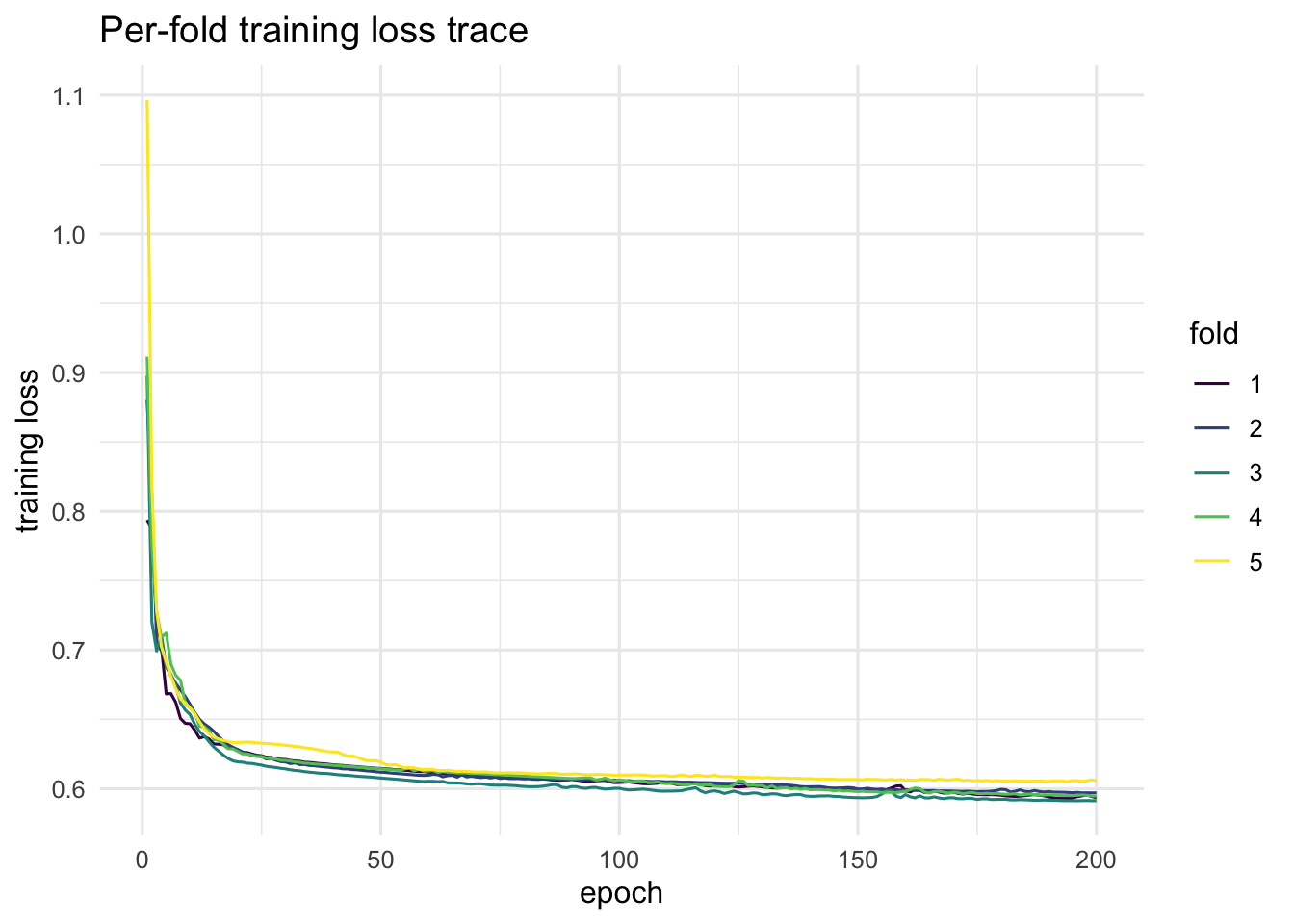
The summary above reports Stage 2: map_c5 — the empirical-Bayes MAP refinement of paper §3. The DML co-partisan coefficient (a large, precisely-estimated positive effect in the paper) is computed from the Stage-1 DNN only; the refined respondent-level betas (used by the distributional and structural quantities below) sit on fit_gs$beta_hat. Pass stage2 = "none" to recover v0.1 behavior.

plot(fit_gs, "loss_trace")

4.3 Population-average estimates

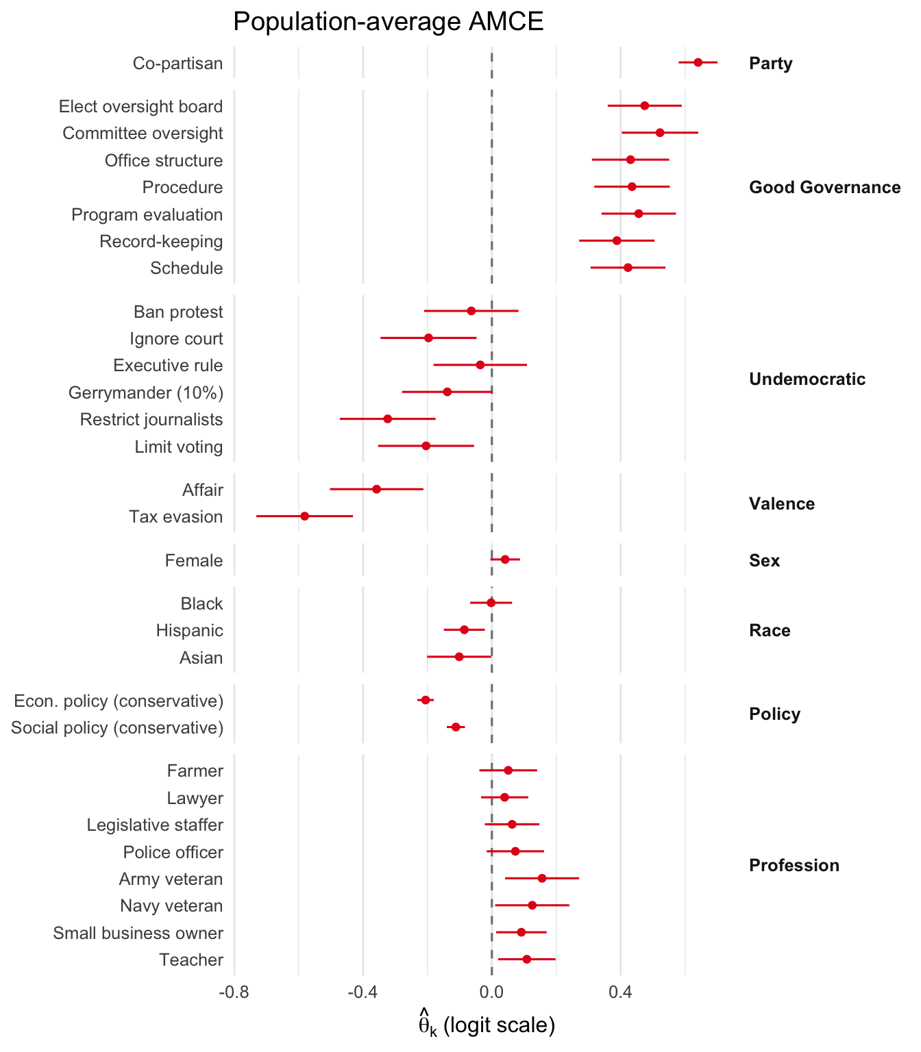
NoteHow to read the AMCE plot

We re-leveled dem_code above so that the reference is u_gerry2 (mild undemocratic action). All dem_code coefficients are now read relative to that baseline:

  • g_* (good-governance) items: positive — voters prefer good-governance practices over mild gerrymandering.
  • Other u_* (undemocratic) items: near zero or negative — similar to or worse than mild gerry.
  • v_* (valence violation) items: strongly negative — voters reject sex affairs / tax evasion even relative to mild undemocratic behavior.

This is the paper’s directional finding: voters favor good governance and oppose democratic backsliding.

Plot the population-average coefficients (DML on the logit scale).

plot_amce(fit_gs, groups = gs_groups, labels = gs_labels)

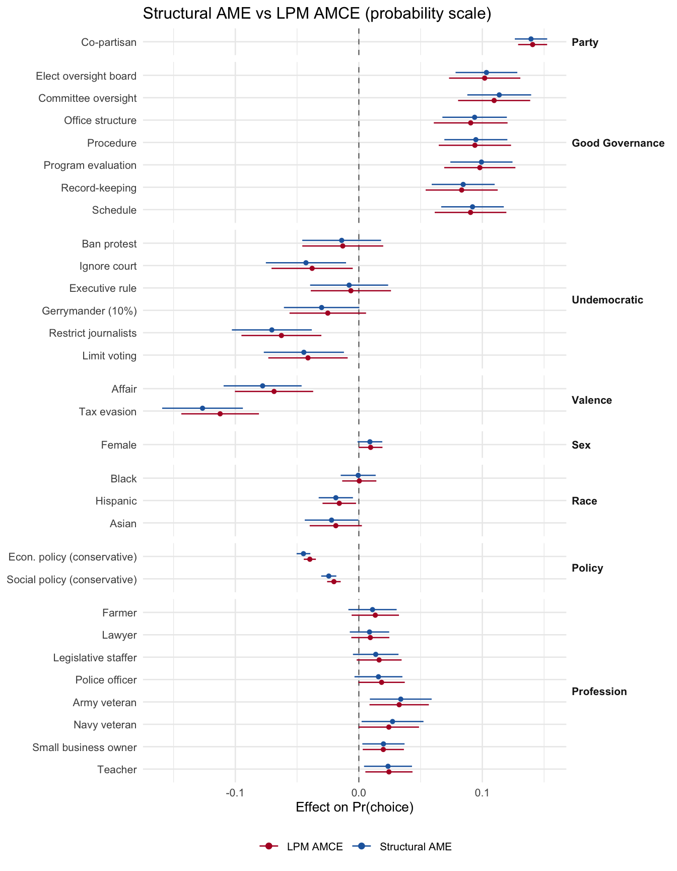
4.3.1 Structural AME vs reduced-form AMCE

Overlay the structural model’s average marginal effects (probability scale) against the linear-probability-model AMCE. Under correct specification the two coincide.

ame_struct <- sc_average(fit_gs, scale = "probability")
ame_df     <- ame_struct$estimate; ame_df$source <- "Structural AME"
lpm        <- sc_baseline_lpm(fit_gs)
amce_df    <- data.frame(
  dummy_name = names(stats::coef(lpm)),
  estimate   = unname(stats::coef(lpm)),
  se         = sqrt(diag(stats::vcov(lpm))),
  source     = "LPM AMCE",
  stringsAsFactors = FALSE
)
amce_df$ci_lo <- amce_df$estimate - 1.96 * amce_df$se
amce_df$ci_hi <- amce_df$estimate + 1.96 * amce_df$se
df_both <- rbind(
  ame_df[, c("dummy_name", "estimate", "se", "ci_lo", "ci_hi", "source")],
  amce_df[, c("dummy_name", "estimate", "se", "ci_lo", "ci_hi", "source")]
)
df_both$label <- ifelse(df_both$dummy_name %in% names(gs_labels),
                        gs_labels[df_both$dummy_name],
                        df_both$dummy_name)
df_both$label <- factor(df_both$label,
                        levels = rev(intersect(unname(gs_labels), df_both$label)))
df_both$group <- gs_groups[df_both$dummy_name]
df_both$group <- factor(df_both$group, levels = unique(gs_groups))
df_both <- df_both[!is.na(df_both$group), ]

ggplot(df_both, aes(x = estimate, y = label, color = source)) +
  geom_vline(xintercept = 0, linetype = "dashed", color = "gray50") +
  geom_pointrange(aes(xmin = ci_lo, xmax = ci_hi),
                  position = position_dodge(width = 0.5),
                  size = 0.3, fatten = 2) +
  scale_color_manual(values = c("Structural AME" = "#2166AC",
                                "LPM AMCE"        = "#B2182B")) +
  facet_grid(group ~ ., scales = "free_y", space = "free_y") +
  labs(x = "Effect on Pr(choice)",
       y = NULL, color = NULL,
       title = "Structural AME vs LPM AMCE (probability scale)") +
  theme_minimal(base_size = 10) +
  theme(legend.position = "bottom",
        strip.text.y    = element_text(angle = 0, hjust = 0, face = "bold"))

4.4 Individual-level preferences

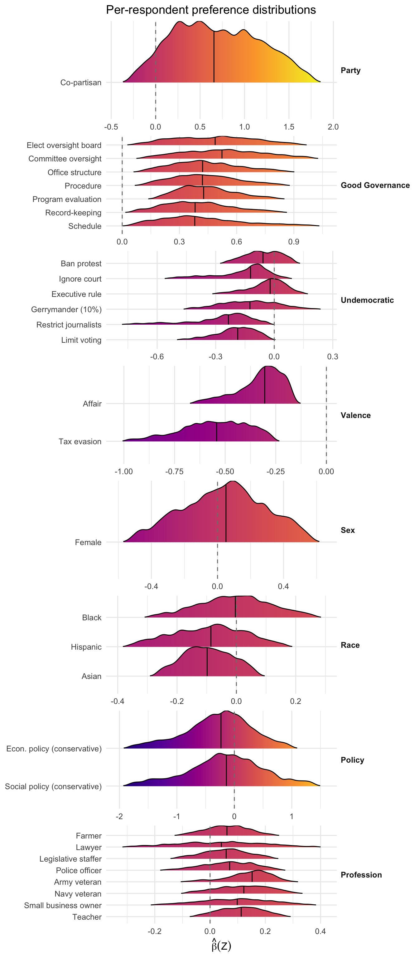
Ridgeline densities show how each per-respondent coefficient \(\hat\beta_k(\mathbf Z_i)\) is distributed across the sample. Undemocratic-action densities should sit entirely left of zero; good-governance densities sit near zero (relative to the g_boardElect reference, see the callout above).

plot(fit_gs, "beta_ridgelines", groups = gs_groups, labels = gs_labels)

4.5 Structural quantities

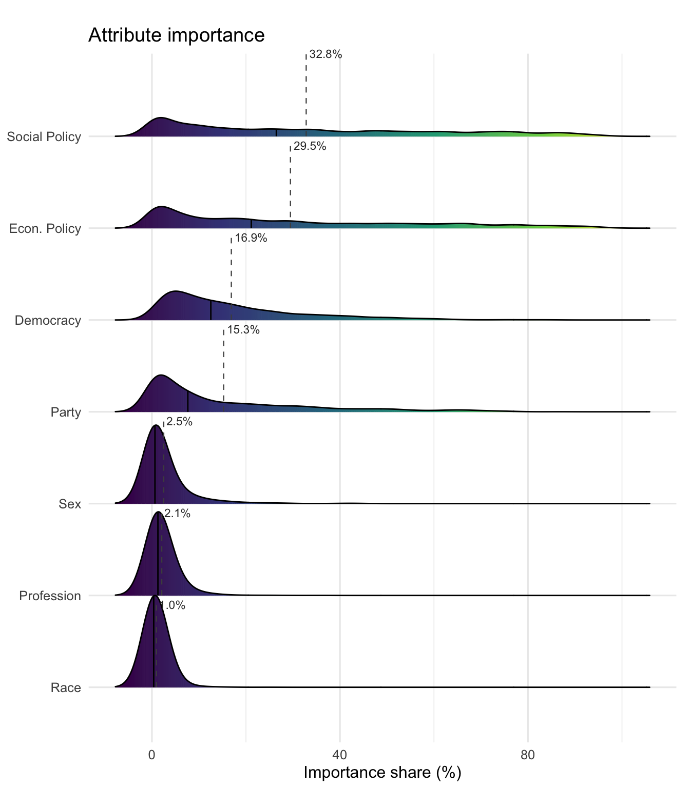
4.5.1 Attribute importance

Decompose utility variance by attribute group. Party and policy should carry most of the weight; democracy attributes should account for a real but smaller share.

sc_importance(fit_gs)
sc_quantity: importance
  estimate: data.frame with 7 rows
  attribute    share        se    ci_lo   ci_hi
 copartisan 0.152848 0.0044524 0.144121 0.16157
         p1 0.294066 0.0067027 0.280929 0.30720
         p2 0.327850 0.0069676 0.314193 0.34151
   dem_code 0.169238 0.0037058 0.161975 0.17650
   cand_sex 0.025320 0.0012235 0.022922 0.02772
  cand_race 0.009615 0.0004233 0.008786 0.01045
   cand_pro 0.021063 0.0006962 0.019698 0.02243
plot_importance(fit_gs, labels = c(copartisan = "Party", p1 = "Econ. Policy",
  p2 = "Social Policy", dem_code = "Democracy",
  cand_sex = "Sex", cand_race = "Race", cand_pro = "Profession"))

4.6 Heterogeneity test

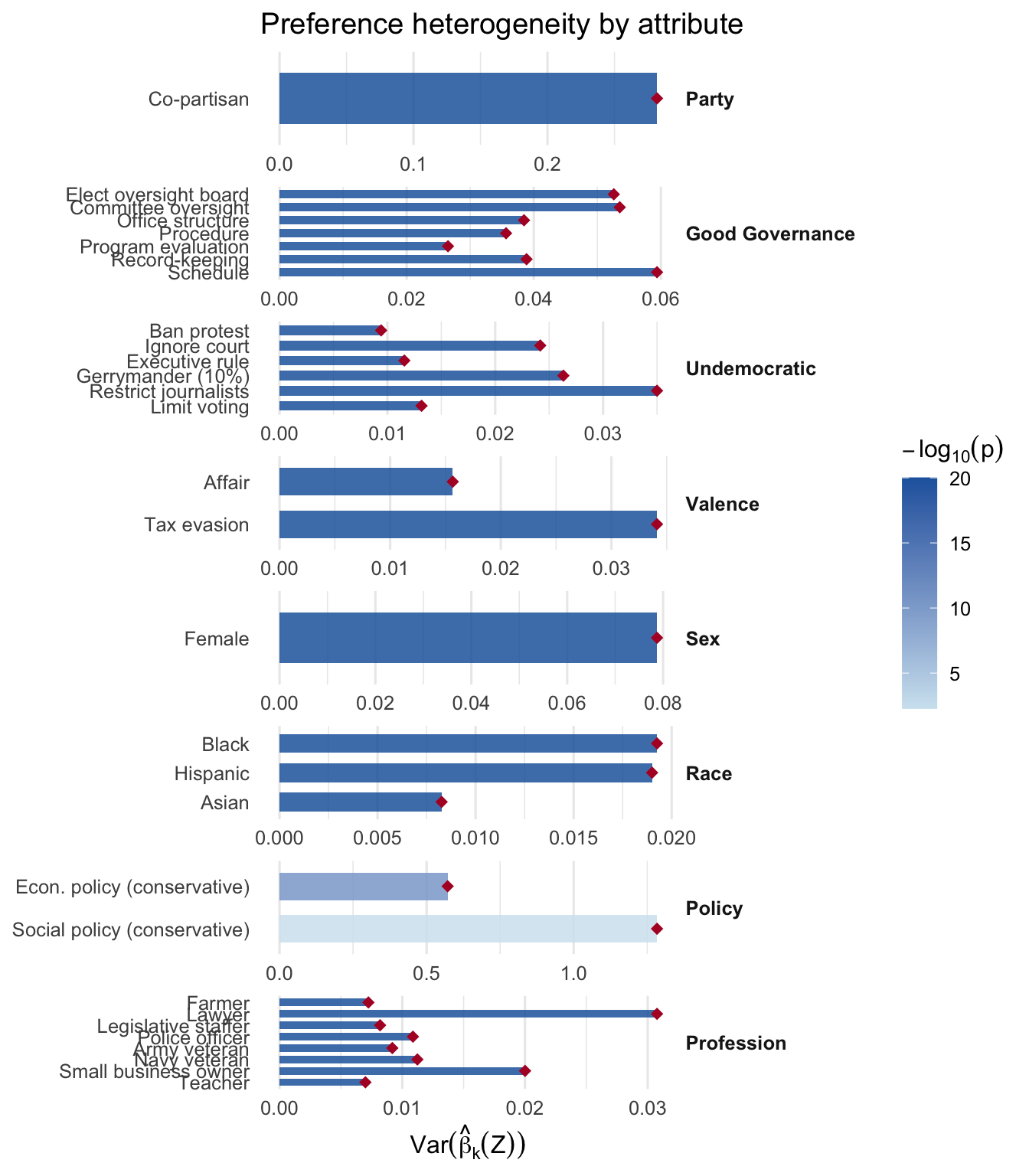
Does the per-attribute dispersion of \(\hat\beta_k(\mathbf Z_i)\) exceed what sampling noise alone would explain? A significant result for undem levels would confirm that the penalty for undemocratic behavior varies meaningfully across respondents.

het_gs <- sc_heterogeneity_test(fit_gs, adjust = "bh")
het_gs$estimate
                     dummy_name    var_beta       se_var    t_stat
1         copartisanCo-partisan 0.281767182 0.0085407929 32.990752
2                            p1 0.571622104 0.0877105300  6.517143
3                            p2 1.283291313 0.5018099339  2.557325
4          dem_codeg_boardElect 0.052589987 0.0016443082 31.983047
5           dem_codeg_committee 0.053526250 0.0017510117 30.568756
6     dem_codeg_officestructure 0.038464517 0.0013614557 28.252492
7           dem_codeg_procedure 0.035640064 0.0012580003 28.330728
8            dem_codeg_progEval 0.026505853 0.0010393435 25.502497
9              dem_codeg_record 0.038862294 0.0014440820 26.911418
10           dem_codeg_schedule 0.059389390 0.0023207196 25.590938
11         dem_codeu_banProtest 0.009420941 0.0003067004 30.717087
12              dem_codeu_court 0.024173119 0.0010061266 24.025921
13           dem_codeu_execRule 0.011573070 0.0005106329 22.664168
14            dem_codeu_gerry10 0.026319789 0.0009877042 26.647440
15        dem_codeu_journalists 0.035000847 0.0017379795 20.138815
16          dem_codeu_limitVote 0.013169032 0.0006100491 21.586839
17             dem_codev_affair 0.015658417 0.0006921117 22.624120
18                dem_codev_tax 0.034122092 0.0012721966 26.821400
19               cand_sexFemale 0.078734915 0.0027861914 28.258975
20               cand_raceBlack 0.019254884 0.0007530385 25.569588
21            cand_raceHispanic 0.019002502 0.0006723982 28.260786
22               cand_raceAsian 0.008269240 0.0002826669 29.254366
23               cand_proFarmer 0.007242420 0.0002644531 27.386403
24               cand_proLawyer 0.030758763 0.0011636483 26.433040
25  cand_proLegislative staffer 0.008194036 0.0002865823 28.592262
26       cand_proPolice officer 0.010869745 0.0003998394 27.185279
27   cand_proServed in the army 0.009190193 0.0004477432 20.525591
28   cand_proServed in the navy 0.011231014 0.0003937156 28.525702
29 cand_proSmall business owner 0.020006552 0.0007071629 28.291291
30              cand_proTeacher 0.006999287 0.0002305519 30.358837
         p_value    p_adjusted sig
1  5.511793e-239 1.653538e-237 ***
2   3.582945e-11  3.706495e-11 ***
3   5.274024e-03  5.274024e-03  **
4  9.382751e-225 1.407413e-223 ***
5  1.592855e-205 1.194641e-204 ***
6  6.632272e-176 1.530524e-175 ***
7  7.230852e-177 2.410284e-176 ***
8  9.247376e-144 1.261006e-143 ***
9  8.073086e-160 1.513704e-159 ***
10 9.622337e-145 1.443351e-144 ***
11 1.683009e-207 1.683009e-206 ***
12 7.453275e-128 9.721663e-128 ***
13 5.057039e-114 6.321299e-114 ***
14 9.581207e-157 1.596868e-156 ***
15  1.686549e-90  1.807016e-90 ***
16 1.193990e-103 1.377680e-103 ***
17 1.254596e-113 1.505515e-113 ***
18 9.095377e-159 1.605067e-158 ***
19 5.520847e-176 1.380212e-175 ***
20 1.662745e-144 2.375350e-144 ***
21 5.245112e-176 1.380212e-175 ***
22 1.975661e-188 9.878304e-188 ***
23 1.991094e-165 4.266629e-165 ***
24 2.858556e-154 4.513509e-154 ***
25 4.192454e-180 1.796766e-179 ***
26 4.848652e-163 9.697304e-163 ***
27  6.360365e-94  7.067072e-94 ***
28 2.812104e-179 1.054539e-178 ***
29 2.211487e-176 6.634460e-176 ***
30 9.604035e-203 5.762421e-202 ***
plot_hetero(fit_gs, groups = gs_groups, labels = gs_labels)

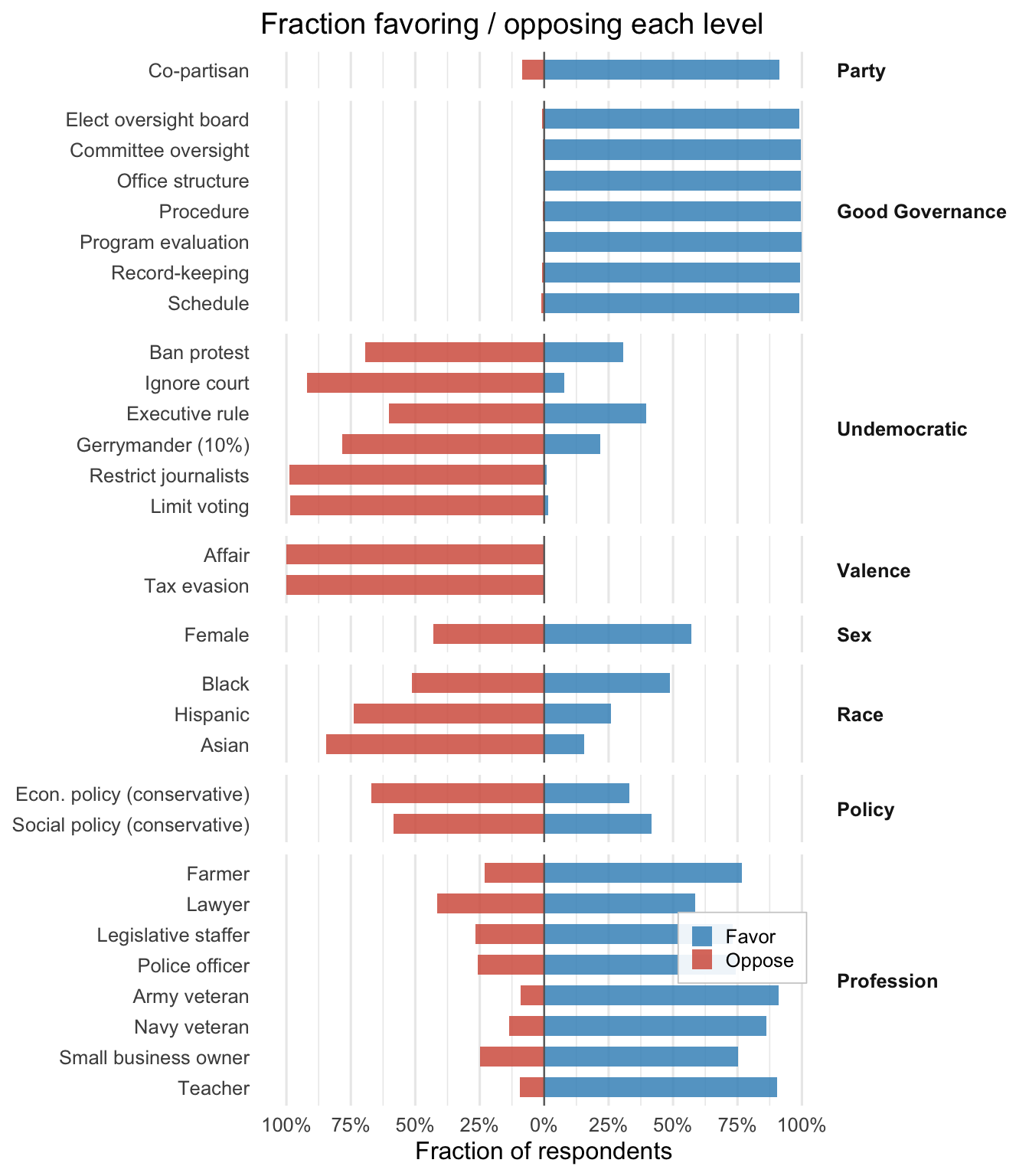
Fewer than 5% of respondents have a positive coefficient on any undemocratic action — opposition to democratic backsliding is near-universal.

4.6.1 Fraction preferring

plot_fraction(fit_gs, groups = gs_groups, labels = gs_labels)

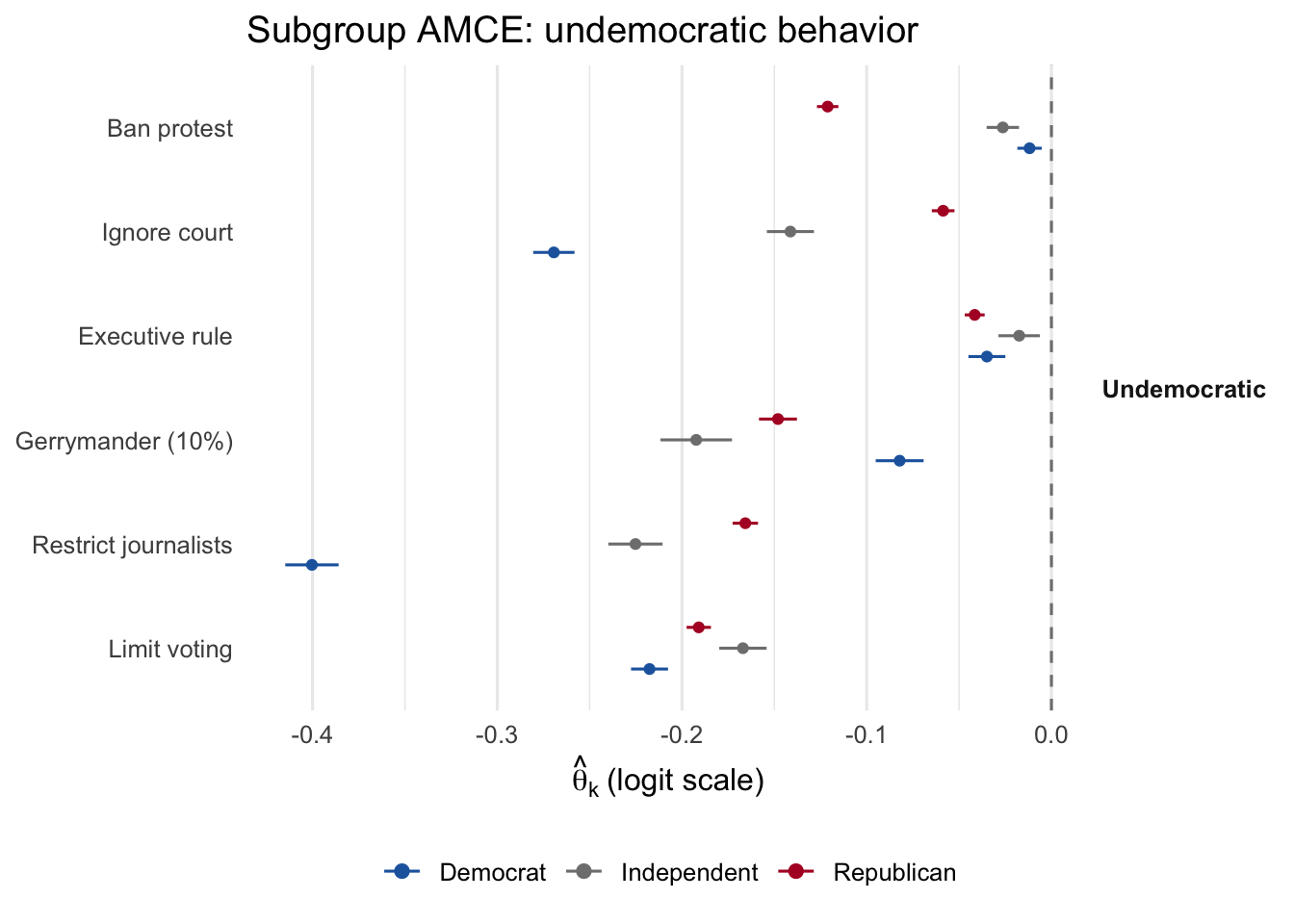
4.7 Direction and intensity

The undemocratic levels should show a large negative average direction (voters penalize them) coupled with high intensity. The structural question is whether the dispersion of those coefficients concentrates on co-partisans, as Graham and Svolik argue.

sc_direction_intensity(fit_gs)
sc_quantity_bivariate: direction_intensity
-- direction --
sc_quantity: direction
  estimate: data.frame with 30 rows
                dummy_name       d     se_d ci_lo_d ci_hi_d
     copartisanCo-partisan  0.8276 0.014083  0.8000  0.8552
                        p1 -0.3396 0.023534 -0.3857 -0.2935
                        p2 -0.1676 0.024664 -0.2160 -0.1193
      dem_codeg_boardElect  0.9824 0.004690  0.9732  0.9916
       dem_codeg_committee  0.9924 0.003078  0.9864  0.9985
 dem_codeg_officestructure  0.9937 0.002811  0.9882  0.9992
       dem_codeg_procedure  0.9912 0.003324  0.9847  0.9977
        dem_codeg_progEval  0.9975 0.001779  0.9940  1.0010
          dem_codeg_record  0.9849 0.004345  0.9764  0.9934
        dem_codeg_schedule  0.9799 0.005011  0.9700  0.9897
  ... 20 more rows
-- intensity --
sc_quantity: intensity
  estimate: data.frame with 30 rows
                dummy_name      u     se_u ci_lo_u ci_hi_u
     copartisanCo-partisan 0.7255 0.012023  0.7019  0.7490
                        p1 0.5608 0.014710  0.5320  0.5896
                        p2 0.6284 0.024087  0.5812  0.6756
      dem_codeg_boardElect 0.4823 0.005702  0.4711  0.4935
       dem_codeg_committee 0.5312 0.005759  0.5199  0.5425
 dem_codeg_officestructure 0.4402 0.004883  0.4306  0.4498
       dem_codeg_procedure 0.4355 0.004706  0.4263  0.4447
        dem_codeg_progEval 0.4460 0.004060  0.4380  0.4540
          dem_codeg_record 0.3984 0.004889  0.3889  0.4080
        dem_codeg_schedule 0.4219 0.006060  0.4100  0.4337
  ... 20 more rows

4.8 Subgroup analysis by partisanship

We re-average the held-out \(\hat\beta(\mathbf Z_i)\) separately for Democrats, Independents, and Republicans using sc_subgroup(). The resp_pid column on the standardized \(\mathbf Z\) matrix preserves the sign of the underlying -1/0/+1 encoding.

pid_col <- fit_gs$Z[, "resp_pid"]
sub <- sc_subgroup(fit_gs, list(
  dem = pid_col < 0,
  ind = pid_col == 0,
  rep = pid_col > 0
))
do.call(rbind, lapply(names(sub), function(g) {
  e <- sub[[g]]$estimate
  rows <- grepl("^dem_codeu_", e$dummy_name)
  data.frame(group = g, e[rows, c("dummy_name", "theta", "se")],
             row.names = NULL)
}))
   group            dummy_name       theta          se
1    dem  dem_codeu_banProtest -0.01182289 0.003384359
2    dem       dem_codeu_court -0.26935861 0.005705399
3    dem    dem_codeu_execRule -0.03493542 0.005096556
4    dem     dem_codeu_gerry10 -0.08215872 0.006613491
5    dem dem_codeu_journalists -0.40033514 0.007367154
6    dem   dem_codeu_limitVote -0.21756876 0.005106420
7    ind  dem_codeu_banProtest -0.02631525 0.004474231
8    ind       dem_codeu_court -0.14131169 0.006501984
9    ind    dem_codeu_execRule -0.01744203 0.005728784
10   ind     dem_codeu_gerry10 -0.19229993 0.009889902
11   ind dem_codeu_journalists -0.22519256 0.007506025
12   ind   dem_codeu_limitVote -0.16700167 0.006539773
13   rep  dem_codeu_banProtest -0.12113598 0.002957310
14   rep       dem_codeu_court -0.05861871 0.003129721
15   rep    dem_codeu_execRule -0.04153361 0.002751085
16   rep     dem_codeu_gerry10 -0.14804233 0.005238231
17   rep dem_codeu_journalists -0.16571228 0.003512436
18   rep   dem_codeu_limitVote -0.19091859 0.003362018
pid_col <- fit_gs$Z[, "resp_pid"]
plot_subgroup(
  fit_gs,
  subgroup = list(Democrat    = pid_col < 0,
                  Independent = pid_col == 0,
                  Republican  = pid_col > 0),
  dummies = grep("^dem_codeu_", fit_gs$attr_names, value = TRUE),
  groups = gs_groups, labels = gs_labels,
  title = "Subgroup AMCE: undemocratic behavior"
)

The structural model reveals that even strong partisans penalize undemocratic behavior, but the intensity of the penalty varies meaningfully with ideology.

4.9 Preference clustering

A complementary view on latent preference types: run k-means on the per-respondent \(\hat\beta(\mathbf Z_i)\) matrix to find clusters of respondents with similar preference profiles.

cl_gs <- sc_clusters(fit_gs, k = 3L, seed = 2024)
cl_gs$estimate$sizes
[1] 8403 3837 8417
round(cl_gs$estimate$centers, 2)
     copartisanCo-partisan    p1    p2 dem_codeg_boardElect
[1,]                  0.76 -0.17  0.07                 0.58
[2,]                  0.98 -0.77 -0.83                 0.74
[3,]                  0.49 -0.20 -0.15                 0.27
     dem_codeg_committee dem_codeg_officestructure dem_codeg_procedure
[1,]                0.62                      0.47                0.49
[2,]                0.81                      0.71                0.68
[3,]                0.32                      0.28                0.27
     dem_codeg_progEval dem_codeg_record dem_codeg_schedule
[1,]               0.46             0.45               0.44
[2,]               0.67             0.66               0.80
[3,]               0.33             0.23               0.23
     dem_codeu_banProtest dem_codeu_court dem_codeu_execRule
[1,]                -0.11           -0.08              -0.04
[2,]                -0.10           -0.42              -0.17
[3,]                 0.01           -0.13               0.03
     dem_codeu_gerry10 dem_codeu_journalists dem_codeu_limitVote
[1,]             -0.21                 -0.17               -0.22
[2,]             -0.20                 -0.56               -0.33
[3,]             -0.01                 -0.26               -0.12
     dem_codev_affair dem_codev_tax cand_sexFemale cand_raceBlack
[1,]            -0.32         -0.60           0.03           0.01
[2,]            -0.52         -0.81           0.12          -0.04
[3,]            -0.25         -0.40           0.02          -0.01
     cand_raceHispanic cand_raceAsian cand_proFarmer cand_proLawyer
[1,]             -0.15          -0.15           0.08           0.02
[2,]             -0.01          -0.12           0.03           0.07
[3,]             -0.08          -0.03           0.05           0.04
     cand_proLegislative staffer cand_proPolice officer
[1,]                        0.00                   0.10
[2,]                        0.13                  -0.05
[3,]                        0.08                   0.09
     cand_proServed in the army cand_proServed in the navy
[1,]                       0.17                       0.18
[2,]                       0.01                       0.17
[3,]                       0.16                       0.03
     cand_proSmall business owner cand_proTeacher
[1,]                         0.14            0.13
[2,]                         0.14            0.13
[3,]                         0.02            0.08

4.10 Validating against the homogeneous-logit AMCE

The structural model nests the standard pooled-logit AMCE: under correct logit specification, \(\theta_k = \mathbb{E}[\beta_k(Z)]\) equals the homogeneous-logit coefficient on attribute \(k\). The new sc_validate_amce() export reports this comparison.

v_gs <- sc_validate_amce(fit_gs)
v_gs
sc_validate_amce -- pooled and (optionally) subgroup comparison
Stage 2: map_c5
N obs: 20657, N respondents: 1605, P attributes: 30
Pooled correlation (DML theta vs homogeneous logit coef): 1

Pooled comparison (first 10 rows):
                 attribute dml_theta dml_se homog_logit_coef homog_logit_se
     copartisanCo-partisan     0.640 0.0307           0.6277        0.00599
                        p1    -0.206 0.0130          -0.1779        0.00250
                        p2    -0.112 0.0143          -0.0907        0.00281
      dem_codeg_boardElect     0.475 0.0586           0.4432        0.01471
       dem_codeg_committee     0.522 0.0606           0.4769        0.01489
 dem_codeg_officestructure     0.431 0.0612           0.3948        0.01523
       dem_codeg_procedure     0.435 0.0598           0.4077        0.01492
        dem_codeg_progEval     0.456 0.0590           0.4262        0.01470
          dem_codeg_record     0.388 0.0597           0.3605        0.01487
        dem_codeg_schedule     0.423 0.0594           0.3923        0.01479
    diff abs_diff
  0.0126   0.0126
 -0.0279   0.0279
 -0.0210   0.0210
  0.0313   0.0313
  0.0452   0.0452
  0.0358   0.0358
  0.0275   0.0275
  0.0297   0.0297
  0.0275   0.0275
  0.0304   0.0304

A correlation near \(r = 1\) across the 30 attribute levels confirms that nothing a reduced-form AMCE analysis would deliver is lost by using the structural model.