data(interflex)
ls()
#>  [1] "app_adiguzel2023" "app_bb2024"       "app_et2023"       "app_hma2015"
#>  [5] "app_vernby2013"   "packages"         "pkg"              "s1"
#>  [9] "s2"               "s3"               "s4"               "s5"
#> [13] "s6"               "s7"               "s8"               "s9"

d<-app_hma2015

## Define variables
Y = "totangry" ## outcome: anger
D = "threat" ## treatment: threat
X = "pidentity" ## moderator: partisan identity
Z <-  c("issuestr2","knowledge", "educ","male", "age10")

Ylabel = "Anger"
Dlabel = "Threat"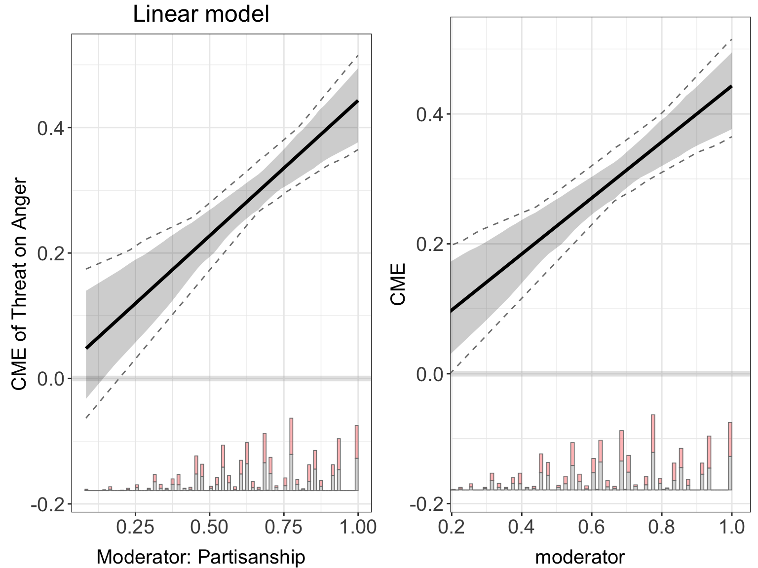
Xlabel = "Partisanship"7 Plot Options
In previous chapter, we have explored most of the plotting options in the interflex package. This chapter serves as a comprehensive guide in plotting CME, using data from Huddy et al. (2015) and simulation data incorporated in the package.
7.1 Load Data
In Huddy et al. (2015), the outcome variable is level of anger, treatment variable is electoral loss threat or electoral win reassurance, and moderator \(X\) is strength of partisan identity. The data is included in the interflex package. We also specify the treatment, outcome, moderator, and controls (covariates).
7.2 The plot function
Users have two equally flexible ways to customise figures produced by interflex:
When setting the option show.all to TRUE in the command plot, the program will return a list in which every element is the plot of one treated group. As all of them are ggplot2 objects, users can then edit those graphs in their ways.
- During estimation: pass any of the plotting-related arguments into
interflex(), then retrieve the figure.
linear.out.1 <- interflex(estimator = "linear", data = d,
                 Y = Y,D = D, X = X, Z = Z,
                 Ylabel = Ylabel, Dlabel = Dlabel,
                 Xlabel = Xlabel, vartype = "bootstrap",
                 main = "Linear model")
#> Parallel computing: using 8 of 14 available cores.
#> To change: set cores = <n> in interflex().
#> Baseline group not specified; choose treat = 0 as the baseline group.
#> Note: Insufficient bootstrap samples (B=200) for Bootstrapped Uniform CI with 50 evaluation points. Using Bonferroni CI by default. Consider increasing nboots for tighter uniform bands.
#> Warning: Using `size` aesthetic for lines was deprecated in ggplot2 3.4.0.
#> ℹ Please use `linewidth` instead.
#> ℹ The deprecated feature was likely used in the interflex package.
#>   Please report the issue to the authors.
linear.out.1$figure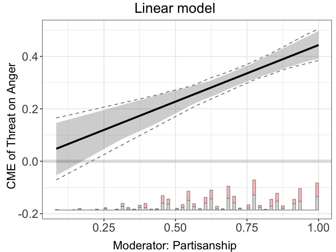
- After estimation: call
plot(result, …)and supply or overwrite the same arguments.
linear.out.1 <- interflex(estimator = "linear", data = d,
                 Y = Y,D = D, X = X, Z = Z,
                 Ylabel = Ylabel, Dlabel = Dlabel,
                 Xlabel = Xlabel, vartype = "bootstrap",
                 main = "Linear model")
#> Parallel computing: using 8 of 14 available cores.
#> To change: set cores = <n> in interflex().
#> Baseline group not specified; choose treat = 0 as the baseline group.
plot(linear.out.1)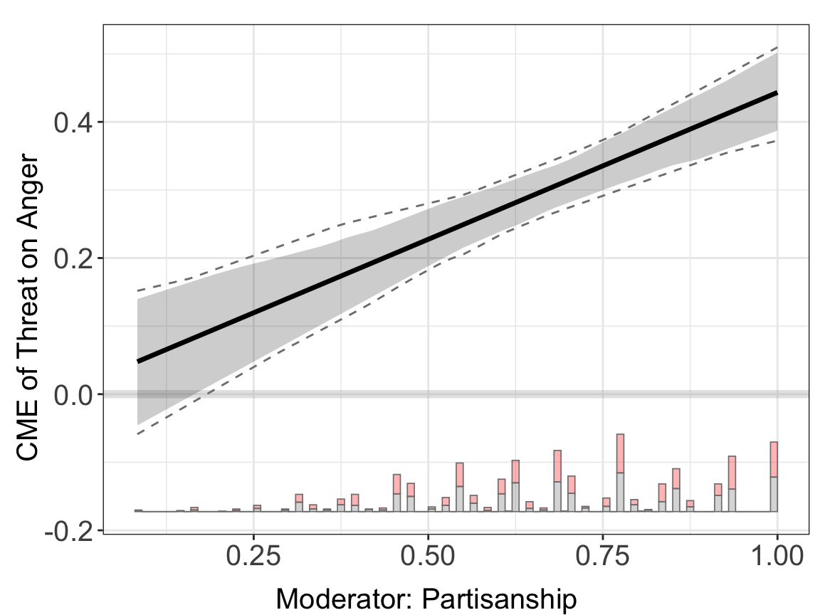
All the options introduced in this chapter are available for both ways.
7.2.1 Estimates to plot
order: For multi-treatment plots: character (discrete treatment) or numeric (continuous) vector that fixes the display order of treatment arms / reference values.
pool: If you supply a list of interflex objects (x), set pool = TRUE to draw a single pooled plot across objects.
For instance, with simulation data s5, by setting the option order and subtitles, users can also specify the order of plots they prefer and the subtitles they want:
By setting pool = TRUE, we can combine these plots. Users can also specify the colors they like:
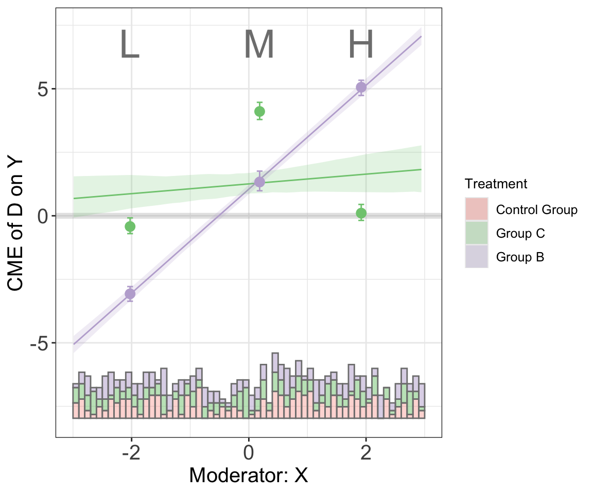
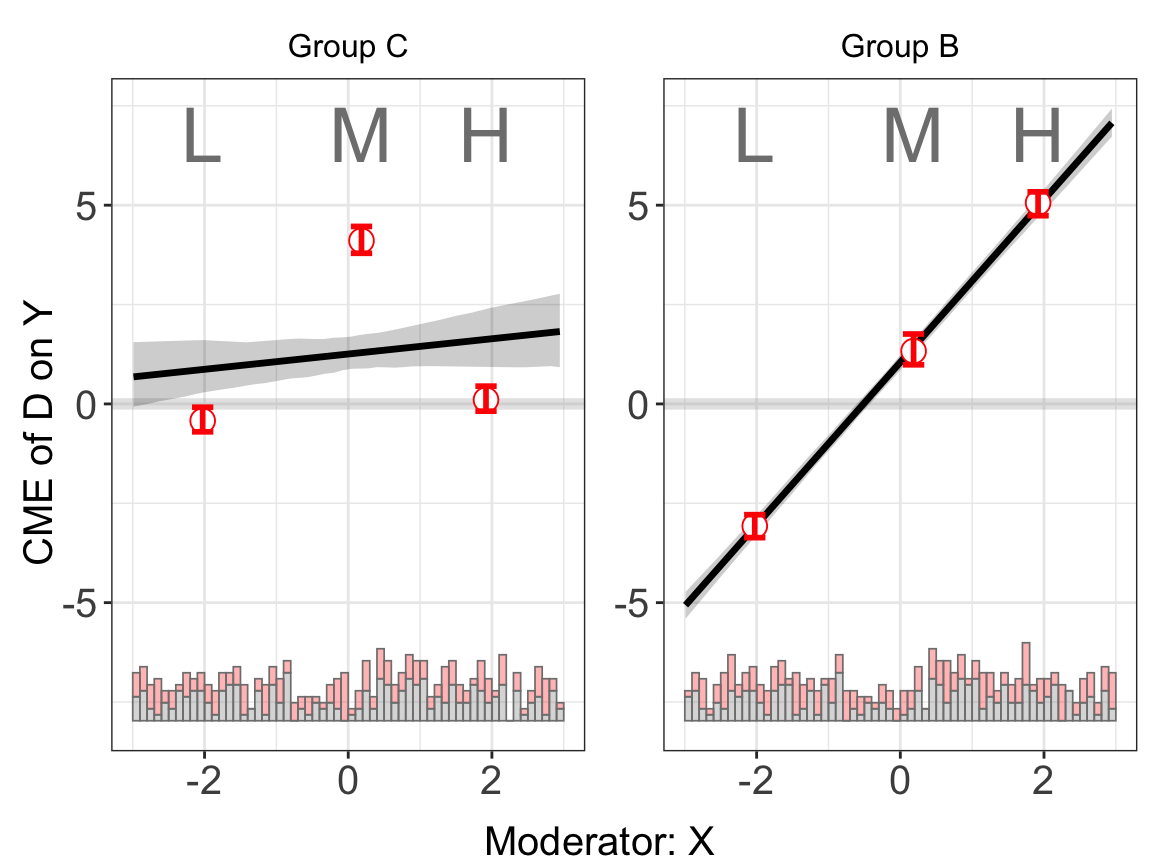
diff.values: interflex allows users to compare treatment effects at three specific values of the moderator using linear or kernel model. In order to do so, users need to pass three values into diff.values when applying linear or kernel estimator.
CI: TRUE / FALSE (or the numeric level) to draw pointwise confidence bands. The default is estimator-dependent (e.g. the kernel estimator uses whatever was saved in the object).
Using the linear estimator with simulation data s5 as an example:
s5.linear <-interflex(Y = "Y", D = "D", X = "X", Z = c("Z1","Z2"),
                      data = s5,
                      estimator = "linear")
#> Baseline group not specified; choose treat = A as the baseline group.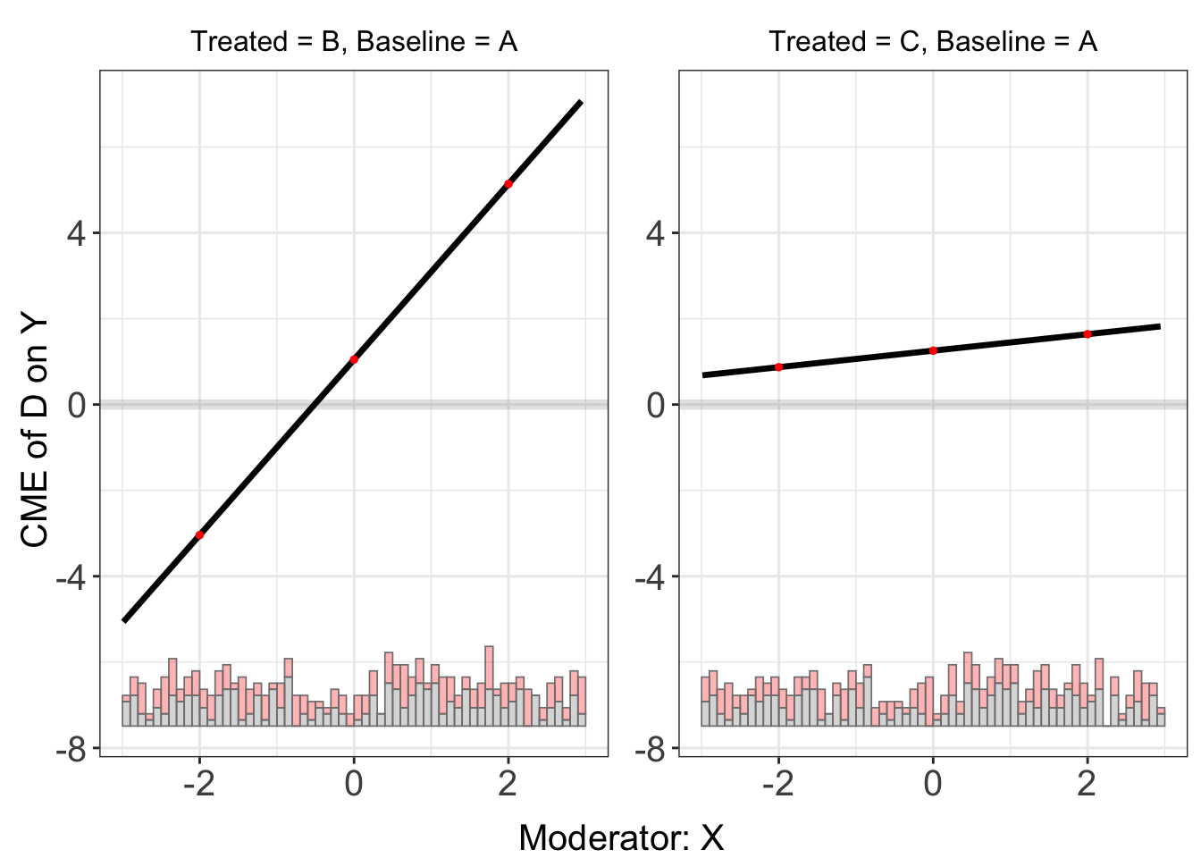
7.2.2 Moderator’s distribution
Xdistr = "histogram": Adds a stacked treatment/control histogram, a shaded marginal density, or nothing beneath the effect curve(s). Options are "histogram", "density", and "none".
hist.color/density.color/hist.color.alpha/density.color.alpha: adjust color and Transparency of the histogram bars / density ribbons.
Using the linear estimation plot with Huddy2015 as an example:
linear.out.1 <- interflex(estimator = "linear", data = d,
                 Y = Y,D = D, X = X, Z = Z,
                 Ylabel = Ylabel, Dlabel = Dlabel,
                 Xlabel = Xlabel, vartype = "bootstrap",
                 main = "Linear model")
#> Parallel computing: using 8 of 14 available cores.
#> To change: set cores = <n> in interflex().
#> Baseline group not specified; choose treat = 0 as the baseline group.

plot(linear.out.1,
     Xdistr = "density",
     density.color = "blue")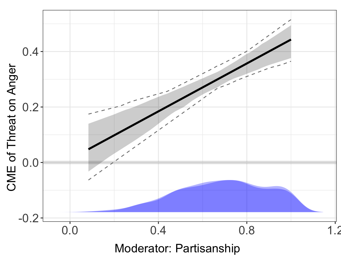
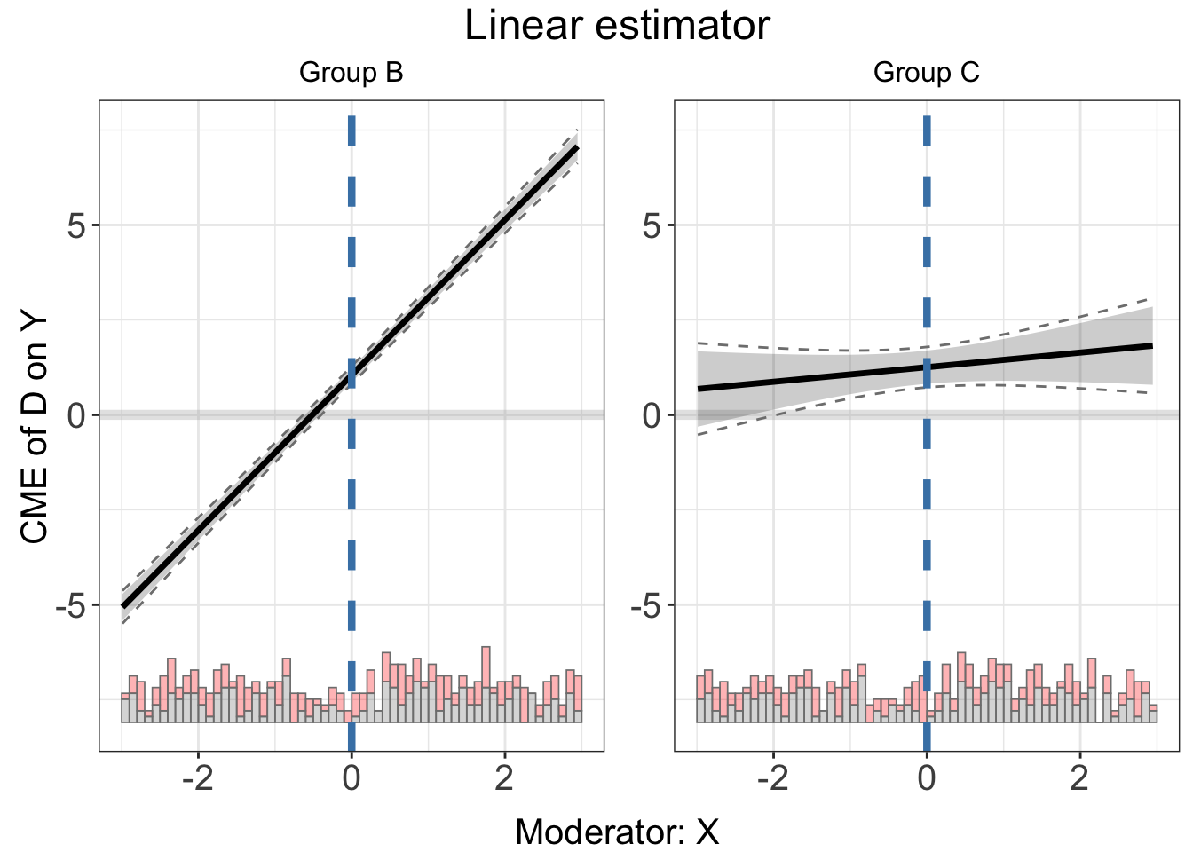
7.2.3 Titles, annotations & facet subtitles
main: Main title (top-center).
subtitles: Vector of custom facet subtitles (length = number of non-baseline treatment arms or reference points).
show.subtitles: Logical; force subtitles on/off irrespective of subtitles or panel count.
interval: Numeric(s); draws light-blue vertical reference line(s) at those moderator values.
legend.title: Title for the legend generated when pool = TRUE.
Using the linear estimation plot with Huddy2015 as an example:
7.2.4 Axis labels & limits
xlab/ylab: Full axis labels (default glue: “Moderator: Xlabel”, “Marginal Effect of Dlabel on Ylabel”).
xlim/ylim: Numeric length-2 vectors to modify the x-axis and y-axis range.
Using the linear estimation plot with Huddy2015, and compare it against the plot without any modification
7.2.5 Theme and layout
theme.bw: TRUE adds theme_bw() and a light grey zero-line; FALSE uses the default ggplot background and a white zero-line.
show.grid: Toggles panel major/minor grid lines.
line.color/line.size: Colour and thickness of the treatment-effect curve(s).
CI.color/CI.color.alpha: Fill colour + alpha for the pointwise CI ribbon.
bin.labs: If you used the binning estimator, prints “L/M/H …” labels underneath each bin centre.
cex.main (title)/cex.sub (subtitle)/cex.lab (axis titles)/cex.axis (tick labels): font size options
ncols: Number of columns when multiple panels are arranged. Defaults to the number of panels.
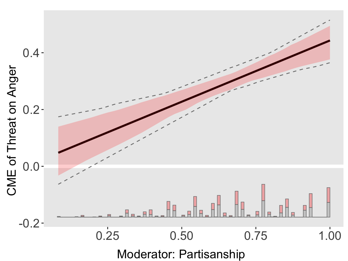
Using the linear estimation plot with Huddy2015 as an example:
plot(linear.out.1, theme.bw = FALSE,
     show.grid = FALSE,
     CI.color = "red")