3 Classic: Extensions
In this chapter, we introduce several extending functions of the binning, linear, and kernel estimator. These extending functions do not depend on the data type of treatment, hence they are applicable to almost all settings. To adopt to the flexibility of these extending function, we use simulation data to illustrate the coding implementation.
s1 is a case of a dichotomous treatment indicator with linear conditional marginal effects (CME); s2 is a case of a continuous treatment indicator with linear CME; s3 is a case of a dichotomous treatment indicator with nonlinear CME; s4 is a case of a dichotomous treatment indicator, nonlinear CME, with additive two-way fixed effects; and s5 is a case of a discrete treatment indicator, nonlinear CME, with additive two-way fixed effects. s1-s5 are generated using the following code:
set.seed(1234)
n<-200
d1<-sample(c(0,1),n,replace=TRUE) # dichotomous treatment
d2<-rnorm(n,3,1) # continuous treatment
x<-rnorm(n,3,1) # moderator
z<-rnorm(n,3,1) # covariate
e<-rnorm(n,0,1) # error term

## linear marginal effect
y1<-5 - 4 * x - 9 * d1 + 3 * x * d1 + 1 * z + 2 * e
y2<-5 - 4 * x - 9 * d2 + 3 * x * d2 + 1 * z + 2 * e
s1<-cbind.data.frame(Y = y1, D = d1, X = x, Z1 = z)
s2<-cbind.data.frame(Y = y2, D = d2, X = x, Z1 = z)

## quadratic marginal effect
x3 <- runif(n, -3,3) # uniformly distributed moderator
y3 <- d1*(x3^2-2.5) + (1-d1)*(-1*x3^2+2.5) + 1 * z + 2 * e
s3 <- cbind.data.frame(D=d1, X=x3, Y=y3, Z1 = z)

## adding two-way fixed effects
n  <- 500
d4 <-sample(c(0,1),n,replace=TRUE) # dichotomous treatment
x4 <- runif(n, -3,3) # uniformly distributed moderator
z4 <- rnorm(n, 3,1) # covariate
alpha <- 20 * rep(rnorm(n/10), each = 10)
xi <- rep(rnorm(10), n/10)
y4 <- d4*(x4^2-2.5) + (1-d4)*(-1*x4^2+2.5) + 1 * z4 +
  alpha + xi + 2 * rnorm(n,0,1)
s4 <- cbind.data.frame(D=d4, X=x4, Y=y4, Z1 = z4, unit = rep(1:(n/10), each = 10), year = rep(1:10, (n/10)))

## Multiple treatment arms
n <- 600
# treatment 1
d1 <- sample(c('A','B','C'),n,replace=T)
# moderator
x <- runif(n,min=-3, max = 3)
# covriates
z1 <- rnorm(n,0,3)
z2 <- rnorm(n,0,2)
# error
e <- rnorm(n,0,1)
y1 <- rep(NA,n)
y1[which(d1=='A')] <- -x[which(d1=='A')]
y1[which(d1=='B')] <- (1+x)[which(d1=='B')]
y1[which(d1=='C')] <- (4-x*x-x)[which(d1=='C')]
y1 <- y1 + e + z1 + z2
s5 <- cbind.data.frame(D=d1, X=x, Y=y1, Z1 = z1,Z2 = z2)
s6 is a case of a dichotomous treatment indicator with the DGP \[E(Y)=prob(Y=1)=logit^{-1}(-1+D+X+DX)=\frac{e^{-1+D+X+DX}}{1+e^{-1+D+X+DX}}\], where D is binary too.
s7 is a case of a continuous treatment indicator with the same DGP as s6 except that D is continuous;
s8 is a case of a dichotomous treatment indicator with nonlinear “linear predictor”: \[E(Y)=prob(Y=1)=logit^{-1}(1+D+X+DX-DX^{2})\]
s9 is a case of a discrete treatment indicator in which for the group 0, \(E(Y)=logit^{-1}(-X)\), for the group 1 \(E(Y)=logit^{-1}(1+X)\), and for the group 2, \(E(Y)=logit^{-1}(-X^{2}-X+4)\).
set.seed(110)
n <- 2000
x <- runif(n,min=-3, max = 3)
d1 <- sample(x = c(0,1),size = n,replace = T)
d2 <- runif(min = 0,max = 1,n = n)
d3 <- sample(x = c(0,1,2),size = n,replace = T)
Z1 <- runif(min = 0,max = 1,n = n)
Z2 <- rnorm(n,3,1)

## s6
link1 <- -1+d1+x+d1*x
prob1 <- exp(link1)/(1+exp(link1))
rand.u <- runif(min = 0,max = 1,n = n)
y1 <- as.numeric(rand.u<prob1)
s6 <- cbind.data.frame(X=x,D=d1,Z1=Z1,Z2=Z2,Y=y1)

## s7
link2 <- -1+d2+x+d2*x
prob2 <- exp(link2)/(1+exp(link2))
rand.u <- runif(min = 0,max = 1,n = n)
y2 <- as.numeric(rand.u<prob2)
s7 <- cbind.data.frame(X=x,D=d2,Z1=Z1,Z2=Z2,Y=y2)

## s8
link3 <- -1+d1+x+d1*x-d1*x*x
prob3 <- exp(link3)/(1+exp(link3))
rand.u <- runif(min = 0,max = 1,n = n)
y3 <- as.numeric(rand.u<prob3)
s8 <- cbind.data.frame(X=x,D=d1,Z1=Z1,Z2=Z2,Y=y3)

## s9
link4 <- rep(NA,n)
link4[which(d3==0)] <- -x[which(d3==0)]
link4[which(d3==1)] <- (1+x)[which(d3==1)]
link4[which(d3==2)] <- (4-x*x-x)[which(d3==2)]

prob4 <- exp(link4)/(1+exp(link4))
rand.u <- runif(min = 0,max = 1,n = n)
y4 <- as.numeric(rand.u<prob4)
s9 <- cbind.data.frame(X=x,D=d3,Z1=Z1,Z2=Z2,Y=y4)
3.1 Fixed effects
First, let’s look at the linear fixed effects models. Remember in s4, a large chunk of the variation in the outcome variable is driven by group fixed effects. Below is a scatterplot of the raw data (group index vs. outcome). Red and green dots represent treatment and control units, respectively. We can see that outcomes are highly correlated within a group.
ggplot() +
  geom_point(data = s4,aes(x = unit, y = Y, colour = as.factor(D))) +
  guides(colour="none") + theme_bw()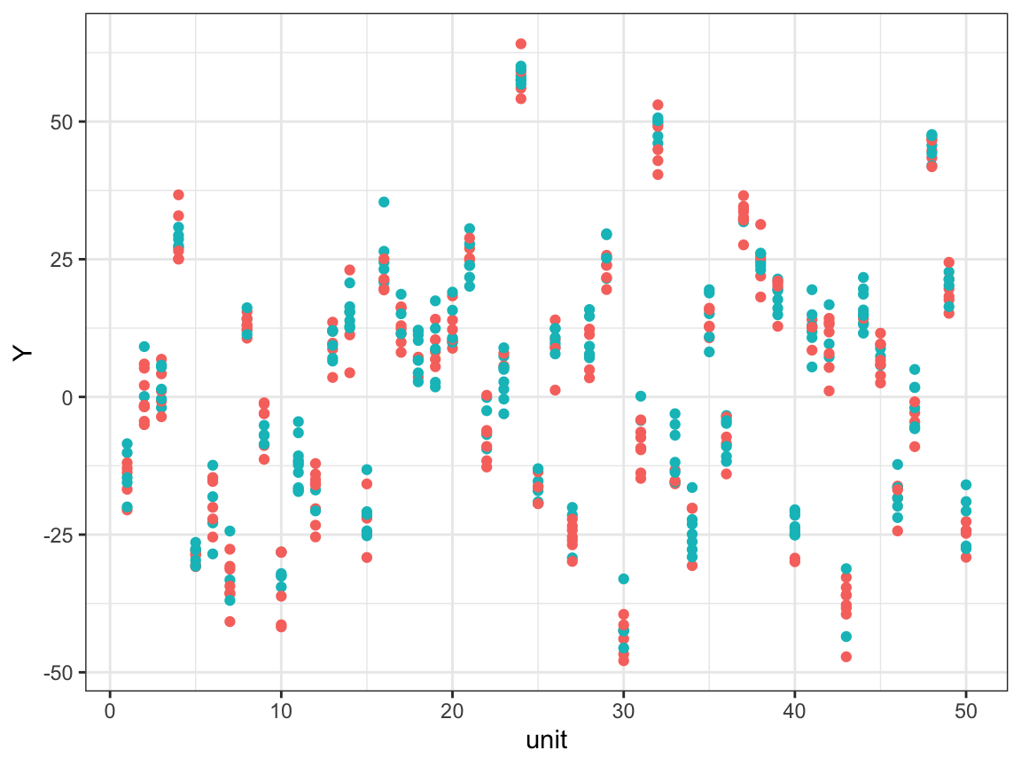
When fixed effects are present, it is possible that we cannot observe a clear pattern of CME in the raw plot as before, while binning estimates have wide confidence intervals:
interflex(estimator = "raw", Y = "Y", D = "D", X = "X", data = s4,
          weights = NULL, ncols=2)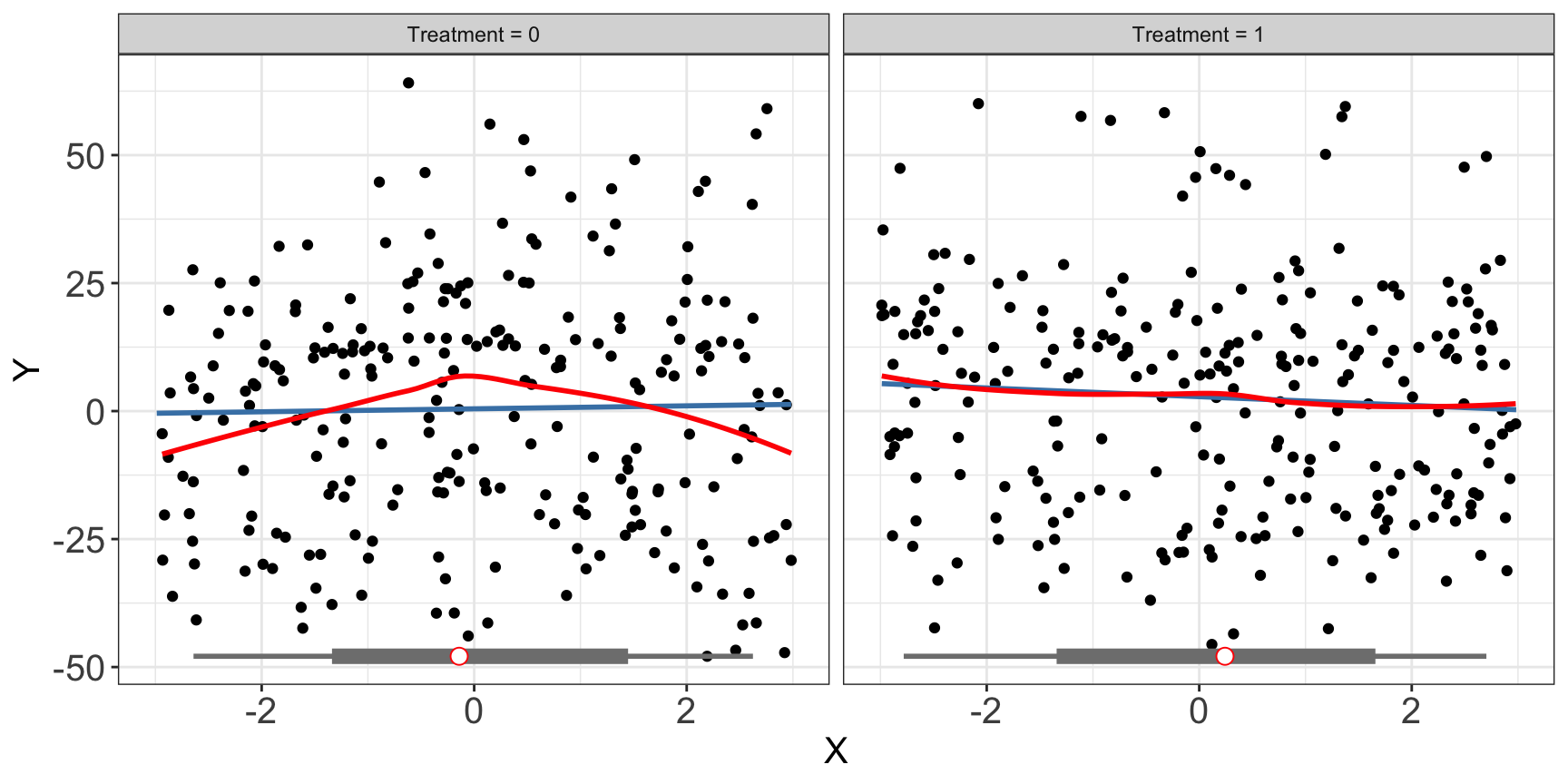
s4.binning <- interflex(Y = "Y", D = "D", X = "X", Z = "Z1", data = s4,
                        estimator = "binning", FE = NULL, cl = "unit")
#> Warning: Using `size` aesthetic for lines was deprecated in ggplot2 3.4.0.
#> ℹ Please use `linewidth` instead.
#> ℹ The deprecated feature was likely used in the interflex package.
#> Please report the issue to the authors.s4.binning$figure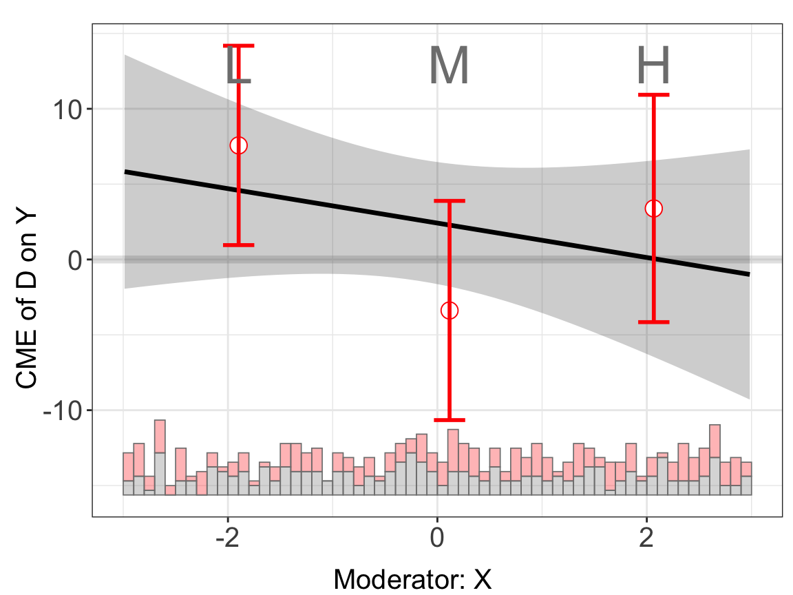
The binning estimates are much more informative when fixed effects are included, by using the FE option. Note that the number of group indicators can exceed 2. Our algorithm is optimized for a large number of fixed effects or many group indicators. The cl option controls the level at which standard errors are clustered.
s4$wgt <- 1
s4.binning <- interflex(Y = "Y", D = "D", X = "X", Z = "Z1", data = s4,
                        estimator = "binning", FE = c("unit", "year"),
cl = "unit", weights = "wgt")s4.binning$figure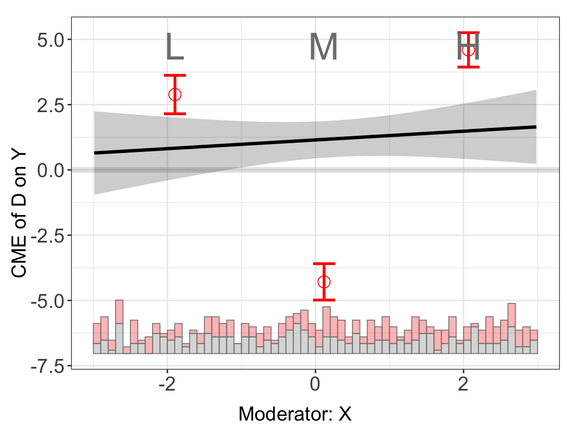
When fixed effects are not taken into account, the kernel estimates are also less precisely estimated. Because the model is incorrectly specified, cross-validated bandwidths also tend to be bigger than optimal.
s4.kernel <- interflex(Y = "Y", D = "D", X = "X", Z = "Z1", data = s4,
                       estimator = "kernel", FE = NULL, vartype = 'bootstrap',
                       nboots = 200, parallel = TRUE,
                       cores = 10,
cl = "unit", weights = "wgt")s4.kernel$figure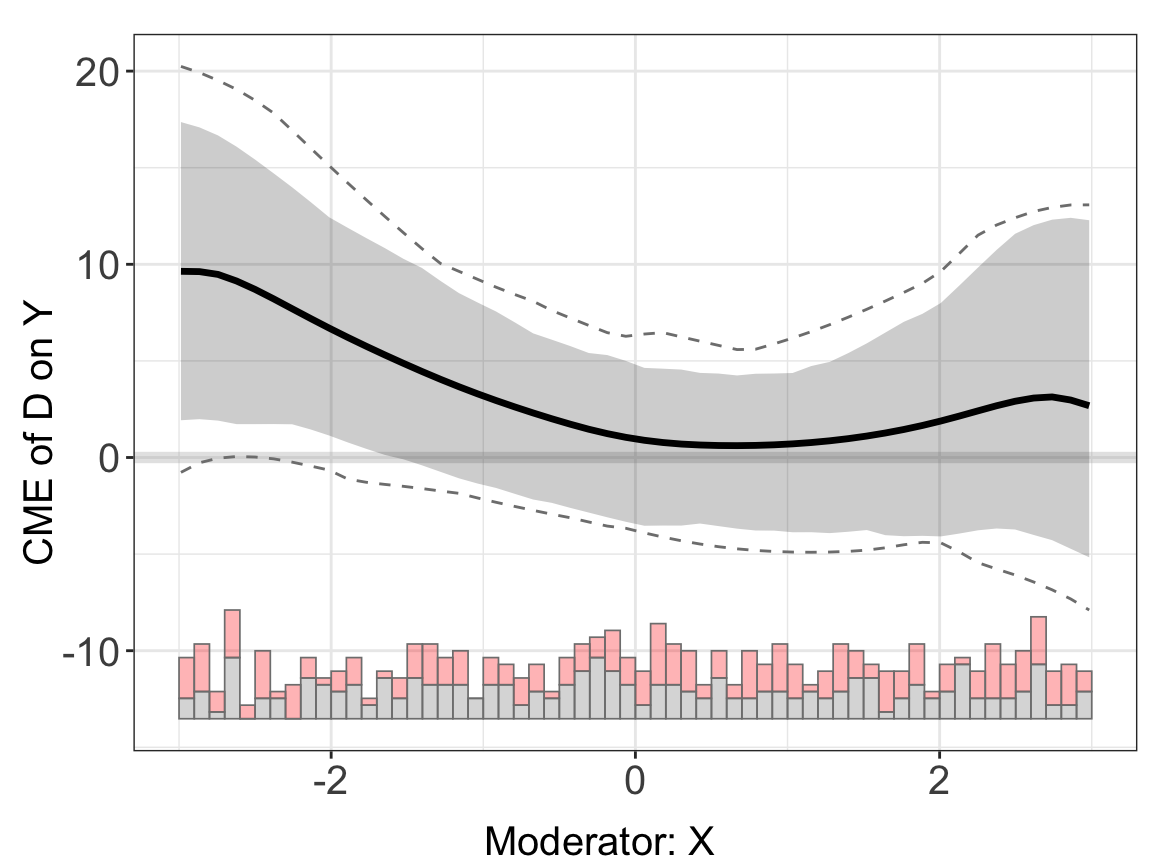
Controlling for fixed effects by using the FE option solves this problem. The estimates are now much closer to the population truth. Note that all uncertainty estimates are produced via bootstrapping. When the cl option is specified, a block bootstrap procedure will be performed.
s4.kernel <- interflex(Y = "Y", D = "D", X = "X", Z = "Z1", data = s4,
                       estimator = "kernel", FE = c("unit","year"), cl = "unit"
                       ,vartype = 'bootstrap',
nboots = 200, parallel = TRUE, cores = 10,weights = "wgt")s4.kernel$figure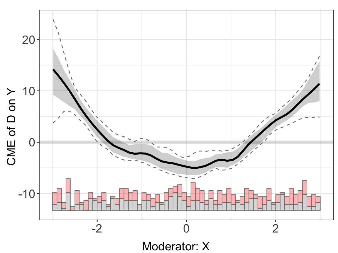
With large datasets, cross-validation or bootstrapping can take a while. One way to check the result quickly is to shut down the bootstrap procedure (using CI = FALSE). interflex will then present the point estimates only. Another way is to supply a reasonable bandwidth manually by using the bw option such that cross-validation will be skipped.
s4.kernel$figure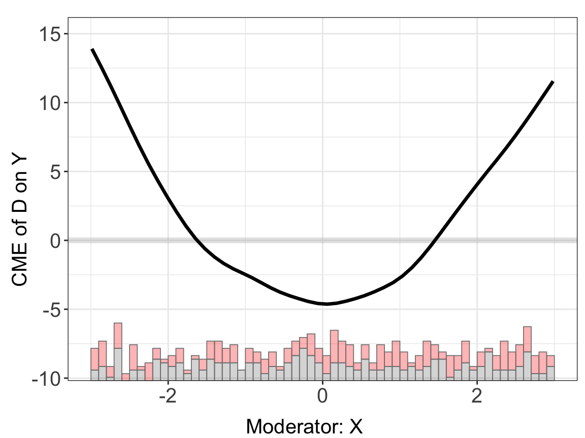
Note that discrete outcome with fixed effects is not supported in the package.
3.2 Multiple treatment arms
Next, we will show how interflex can be applied when there are more than two condition. First, we plot the raw data:
interflex(estimator = "raw",Y = "Y", D = "D", X = "X", data = s5, ncols = 3)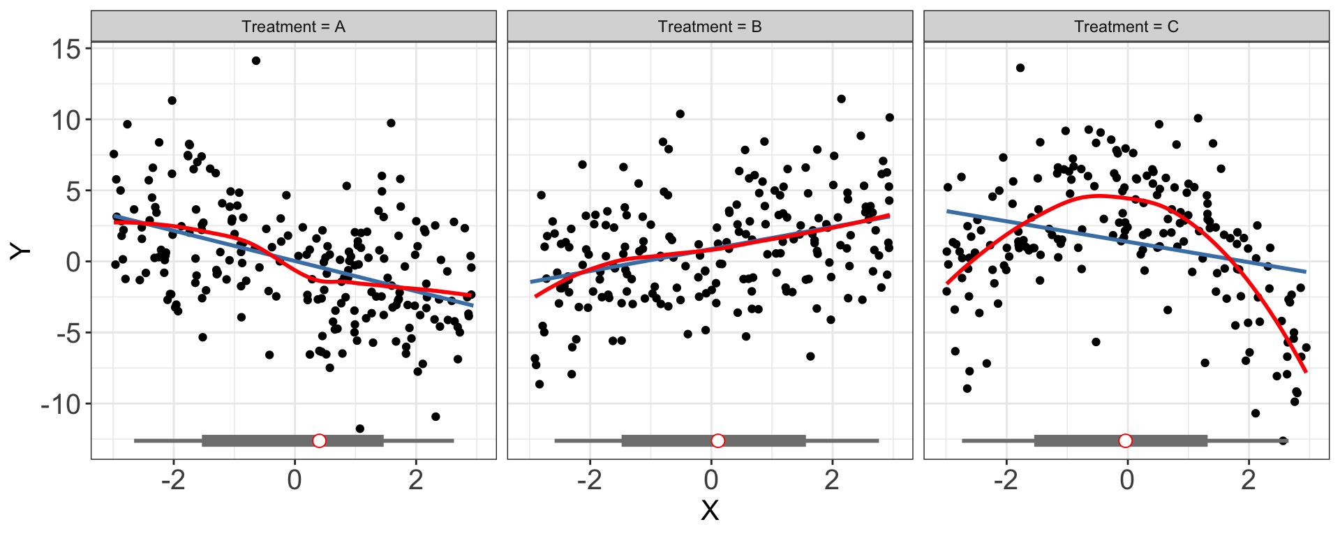
By default, interflex will produce \((n-1)\) CME plots, taking one category as the baseline (if not specified, the base group is selected based on the numeric/character order of the treatment values). Here we also specify vartype = "bootstrap" in order to estimate the confidence intervals.
s5.binning <- interflex(Y = "Y", D = "D", X = "X", Z = c("Z1","Z2"), data = s5,
estimator = "binning", vartype = "bootstrap")s5.binning$figure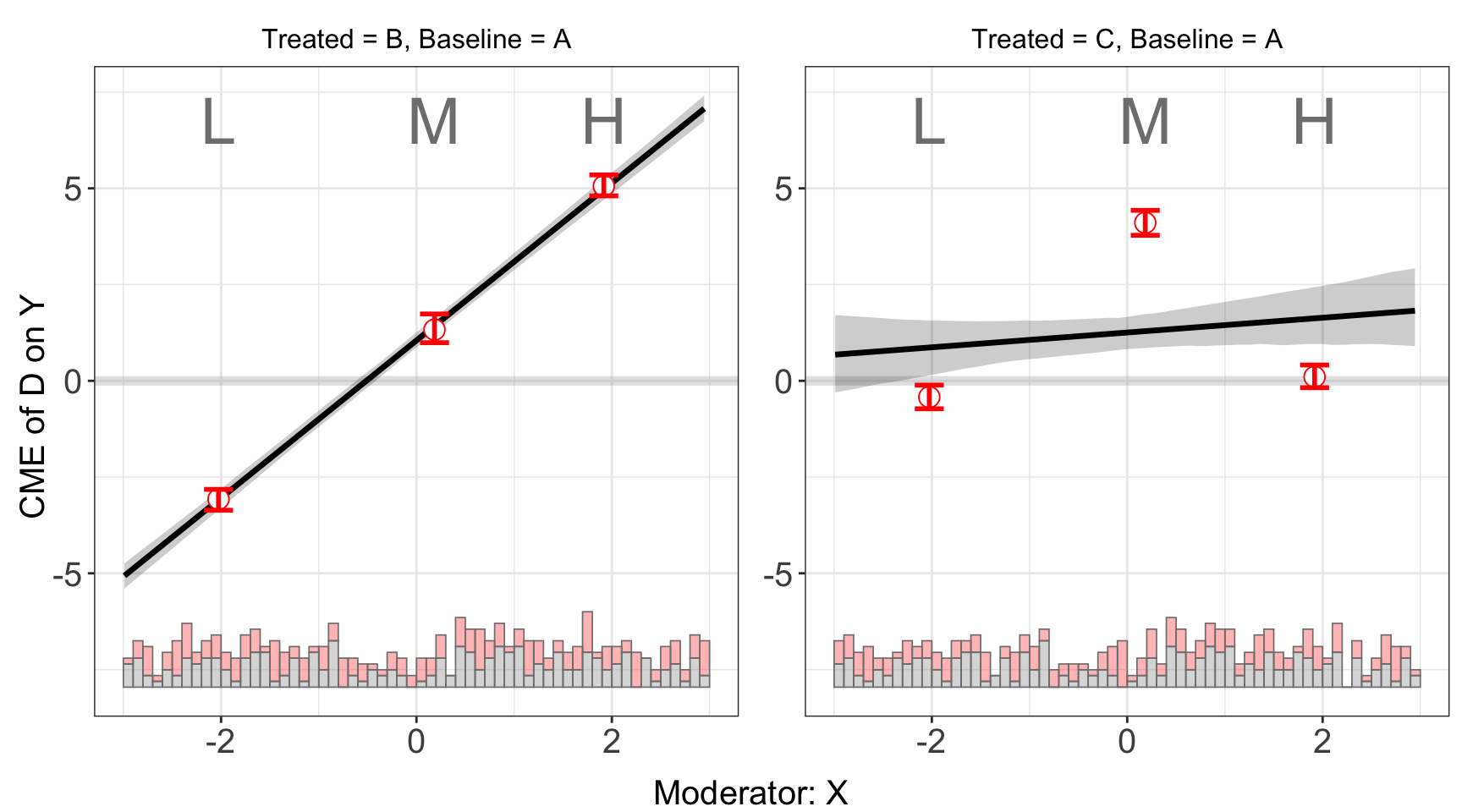
We specify the base group using the option base:
s5.binning2 <- interflex(Y = "Y", D = "D", X = "X",Z = c("Z1", "Z2"), data = s5,
estimator = "binning", base = "B", vartype = "bootstrap")plot(s5.binning2)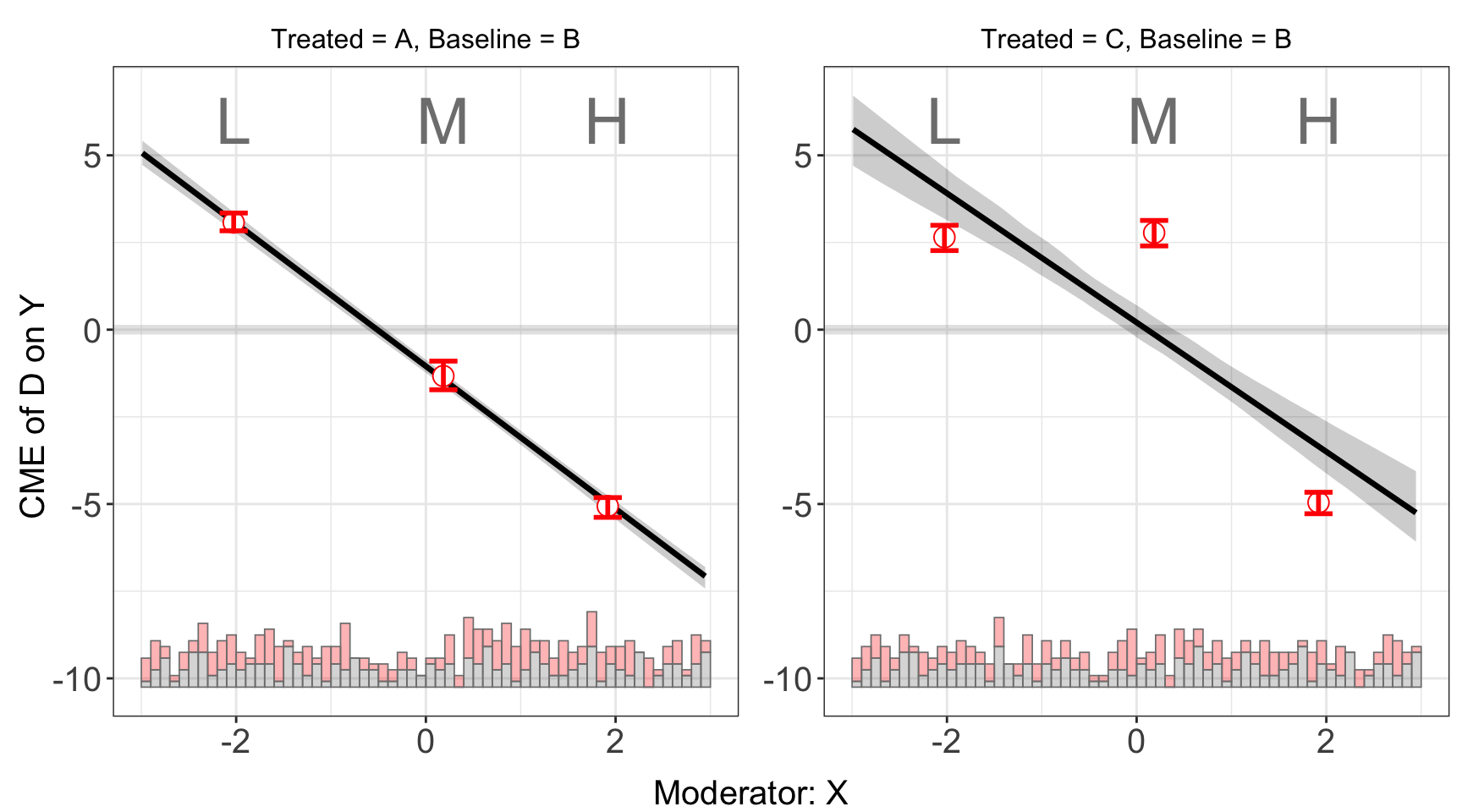
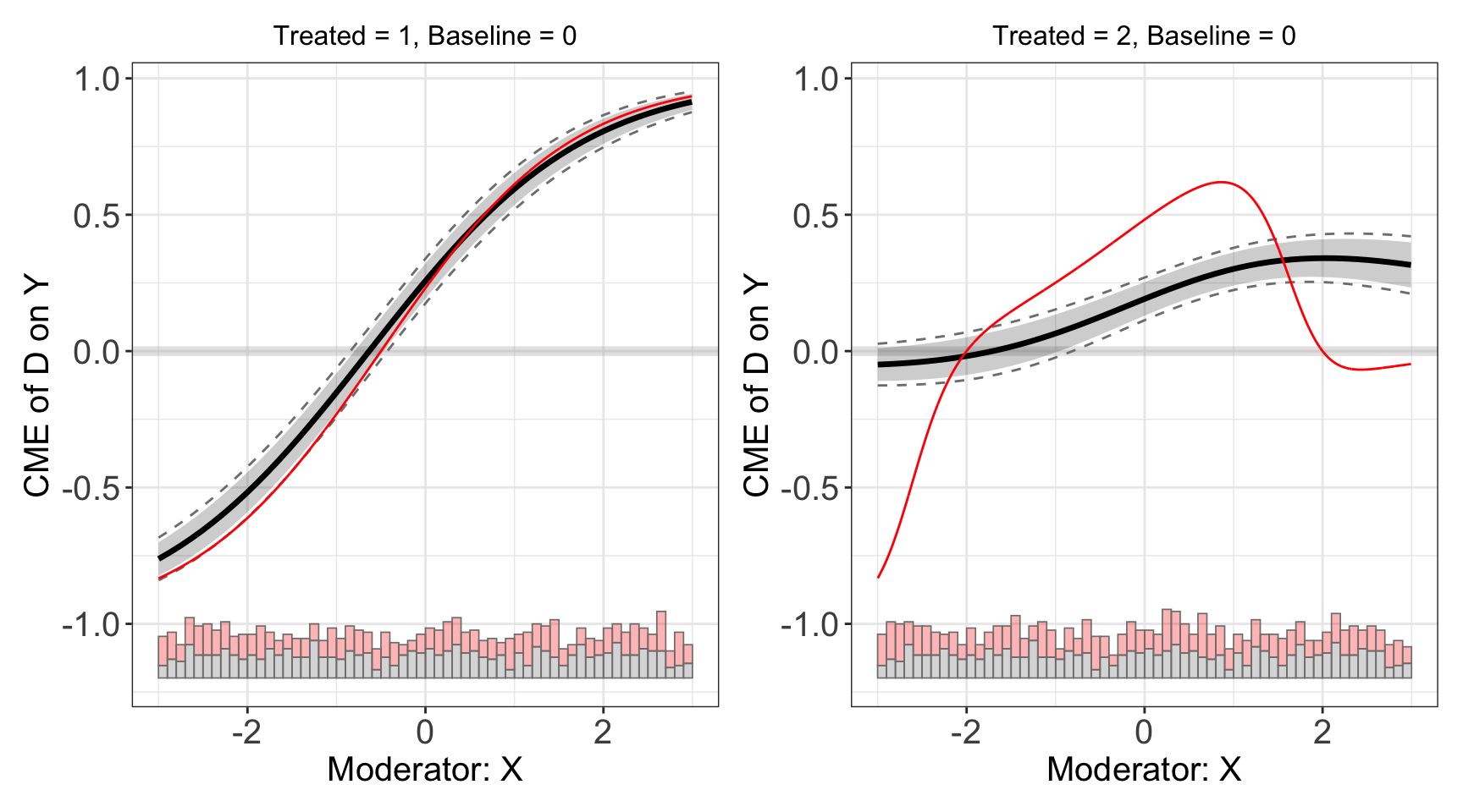
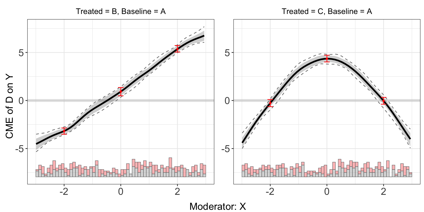
For dataset s5, because of the nonlinear interaction effects, the kernel estimator will produce CME estimates that are much closer to the effects implied by the true DGP.
s5.kernel <- interflex(Y = "Y", D = "D", X = "X",Z = c("Z1", "Z2"), data = s5,
                       estimator = "kernel", vartype = 'bootstrap',
nboots = 200, parallel = TRUE, cores = 10)s5.kernel$figure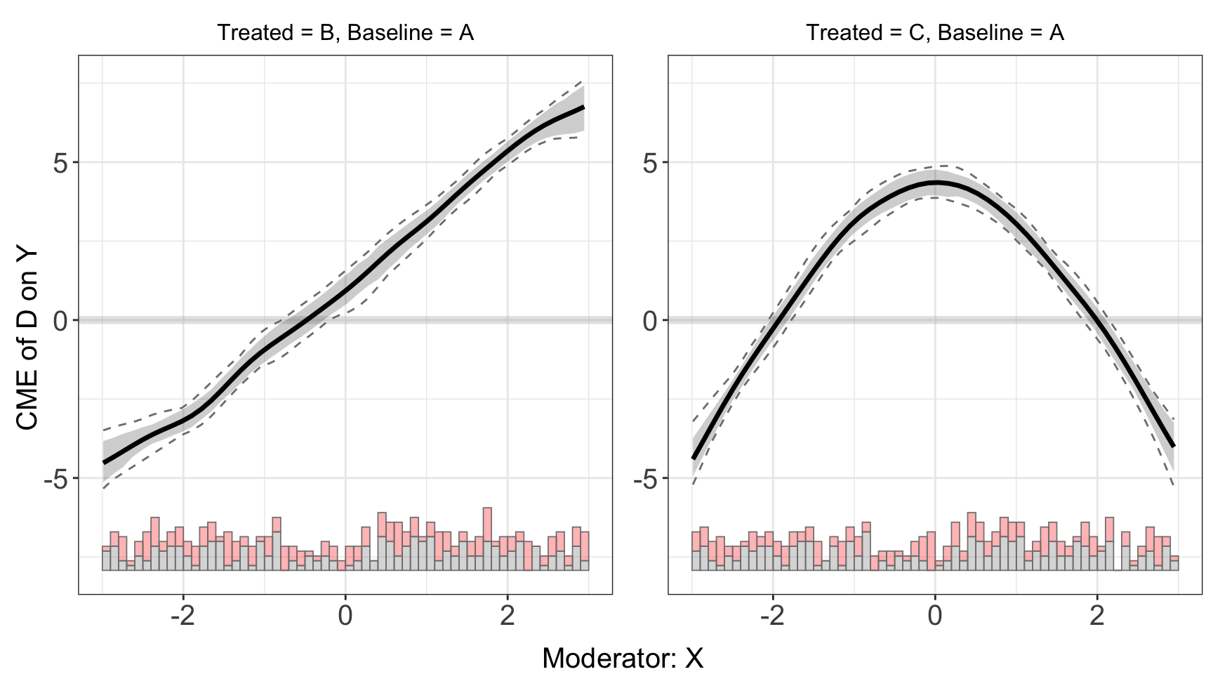
The function can be applied to discrete outcome settings. For s9, the LIE assumption are violated only in group 2. The linear estimator can give a consistent estimation of treatment effects for the group 1, but not group 2.
s9.linear <- interflex(estimator='linear', data=s9, method='logit',
Y = 'Y', D = 'D', X = 'X', Z = c('Z1','Z2'))plot(s9.linear)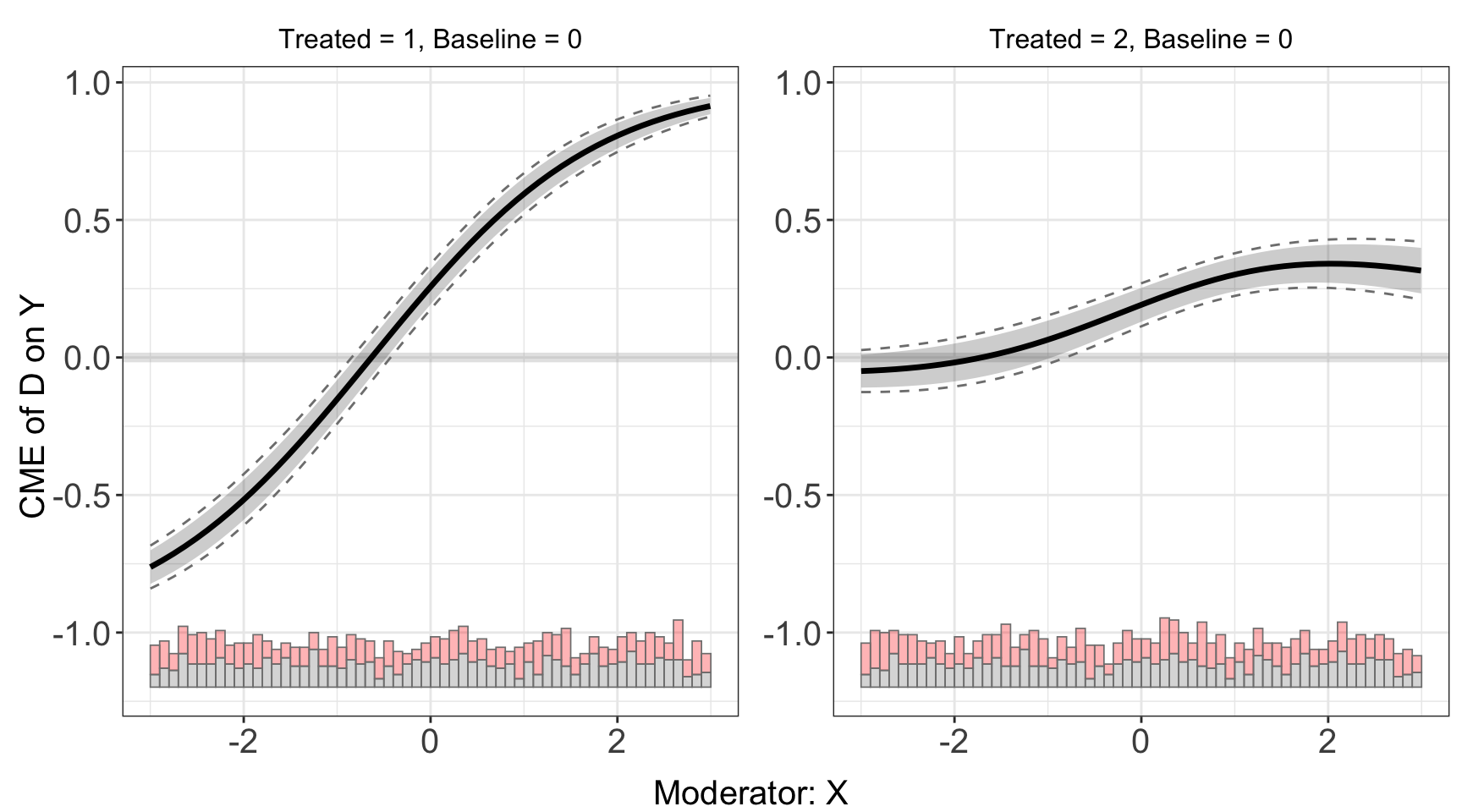
Then, we use the binning estimator to conduct a diagnostic analysis.
s9.binning <- interflex(estimator = 'binning', data = s9, method='logit',
Y = 'Y', D = 'D', X = 'X', Z = c('Z1','Z2'))plot(s9.binning)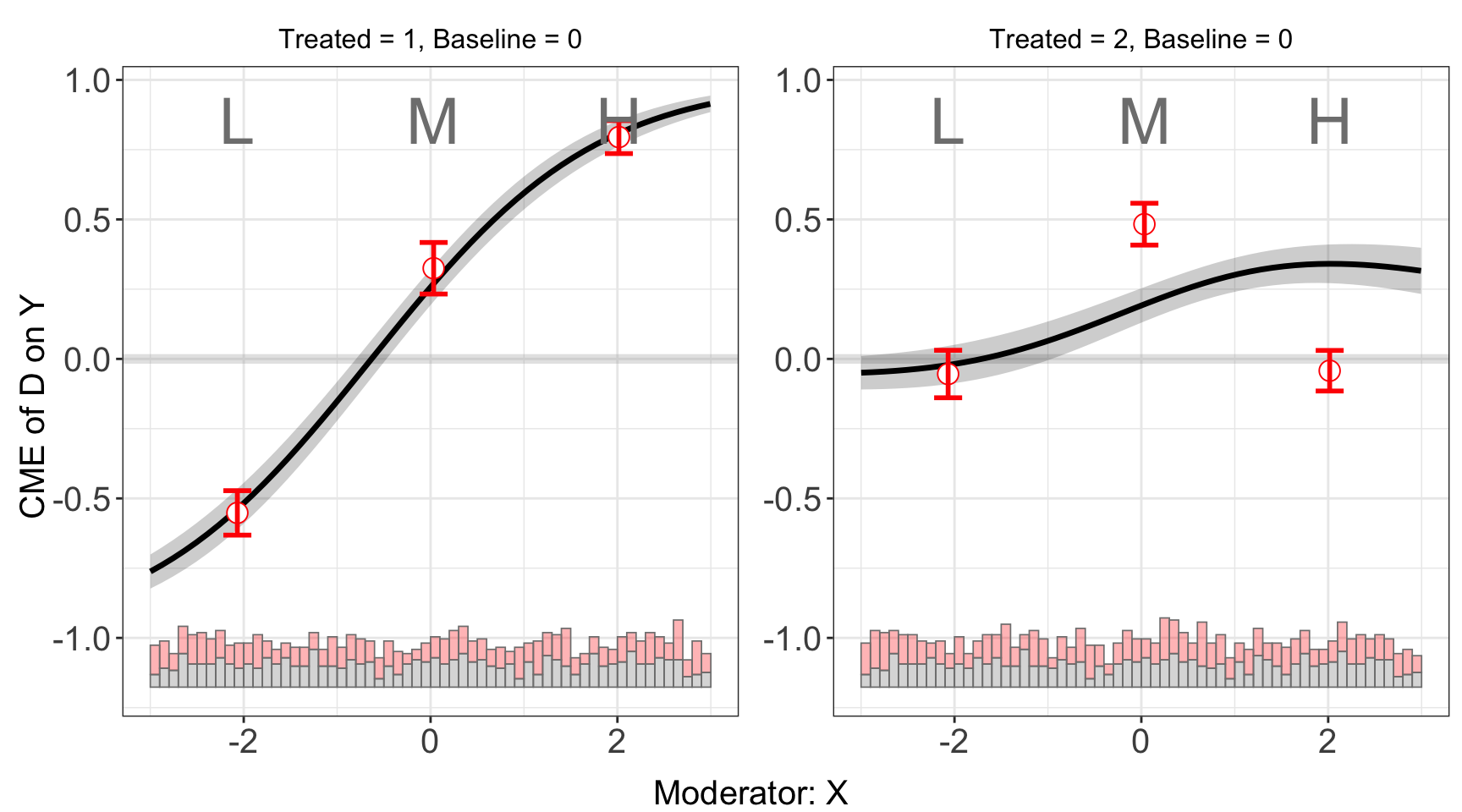
Results of the binning estimator also suggests the violation of LIE for group 2, which can be further verified by checking the test results.
s9.binning$tests$p.wald
#> [1] "0.000"
s9.binning$tests$p.lr
#> [1] "0.000"
Both of these tests suggest that LIE assumption fails in the model, but it doesn’t tell us in which group the assumption fails. There is an extra output “sub.test” when there are more than 3 groups in the data, which includes by-group results of the Wald/Likelihood ratio test, which test the linear multiplicative interaction assumption for each group. In this case, the test results suggest that there are not enough evidences to reject the null hypothesis for group 1, but for group 2, the null hypothesis can be safely rejected.
head(s9.binning$tests$sub.test[[1]])
#> $p.wald
#> [1] "0.195"
#>
#> $p.lr
#> [1] "0.193"
#>
#> $formula.restrict
#> Y ~ X + D.Group.2 + DX.Group.2 + D.Group.3 + DX.Group.3 + Z1 +
#>     Z2 + G.2 + G.2.X + D.Group.3.G.2 + DX.Group.3.G.2 + G.3 +
#>     G.3.X + D.Group.3.G.3 + DX.Group.3.G.3
#> <environment: 0x138dc16d0>
#>
#> $formula.full
#> Y ~ X + D.Group.2 + DX.Group.2 + D.Group.3 + DX.Group.3 + Z1 +
#>     Z2 + G.2 + G.2.X + D.Group.2.G.2 + DX.Group.2.G.2 + D.Group.3.G.2 +
#>     DX.Group.3.G.2 + G.3 + G.3.X + D.Group.2.G.3 + DX.Group.2.G.3 +
#>     D.Group.3.G.3 + DX.Group.3.G.3
#> <environment: 0x138dc16d0>
Lastly, we can use the kernel estimator to get more consistent results.
s9.kernel <- interflex(estimator = 'kernel', data = s9,
                       Y ='Y', D = 'D', X = 'X', Z = c('Z1','Z2'),
                       method='logit',vartype = "bootstrap",
nboots = 200, parallel = TRUE, cores = 10)plot(s9.kernel)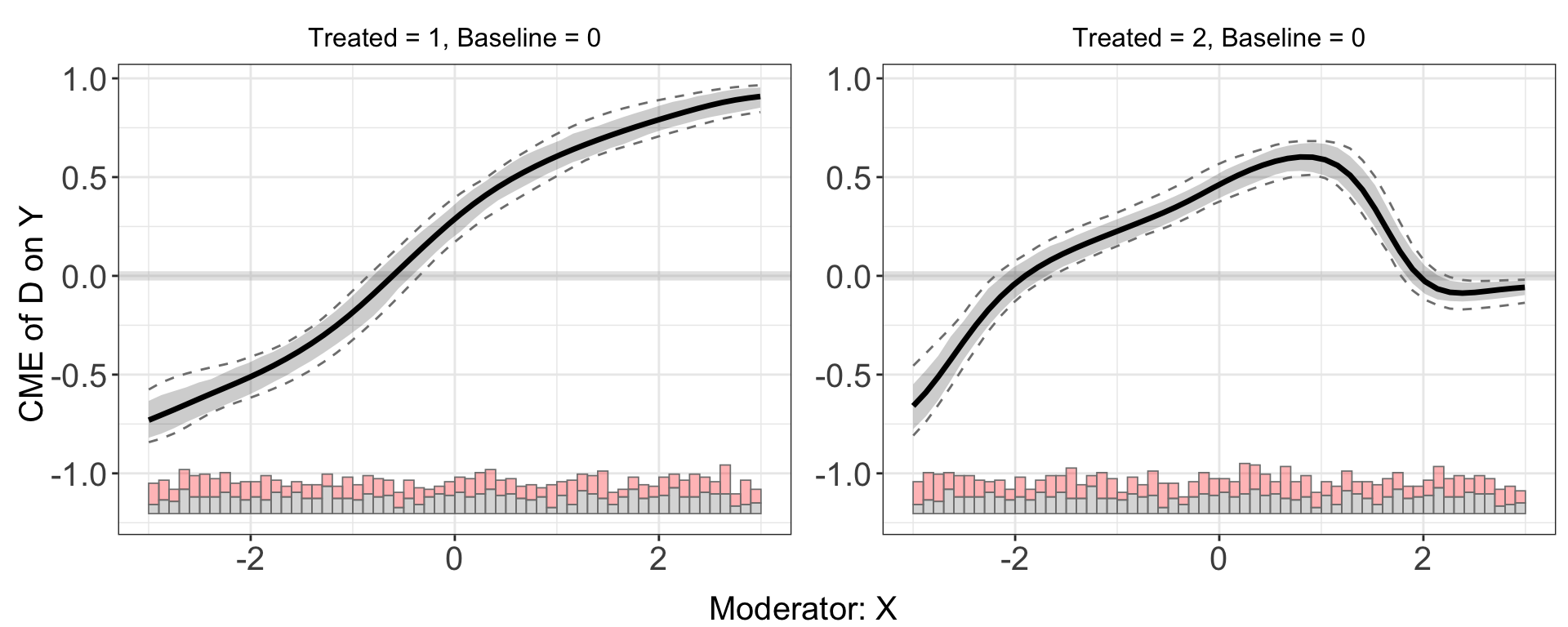
The estimated ATE and \(E(Y|D,X,Z)\) are also grouped by treatment.
s9.kernel$Avg.estimate
#> $`1`
#>                            ATE    sd z-value p-value lower CI(95%)
#> Average Treatment Effect 0.175 0.031   5.735   0.000         0.114
#>                          upper CI(95%)
#> Average Treatment Effect         0.227
#>
#> $`2`
#>                            ATE    sd z-value p-value lower CI(95%)
#> Average Treatment Effect 0.150 0.025   5.904   0.000         0.101
#>                          upper CI(95%)
#> Average Treatment Effect 0.194predict(s9.kernel)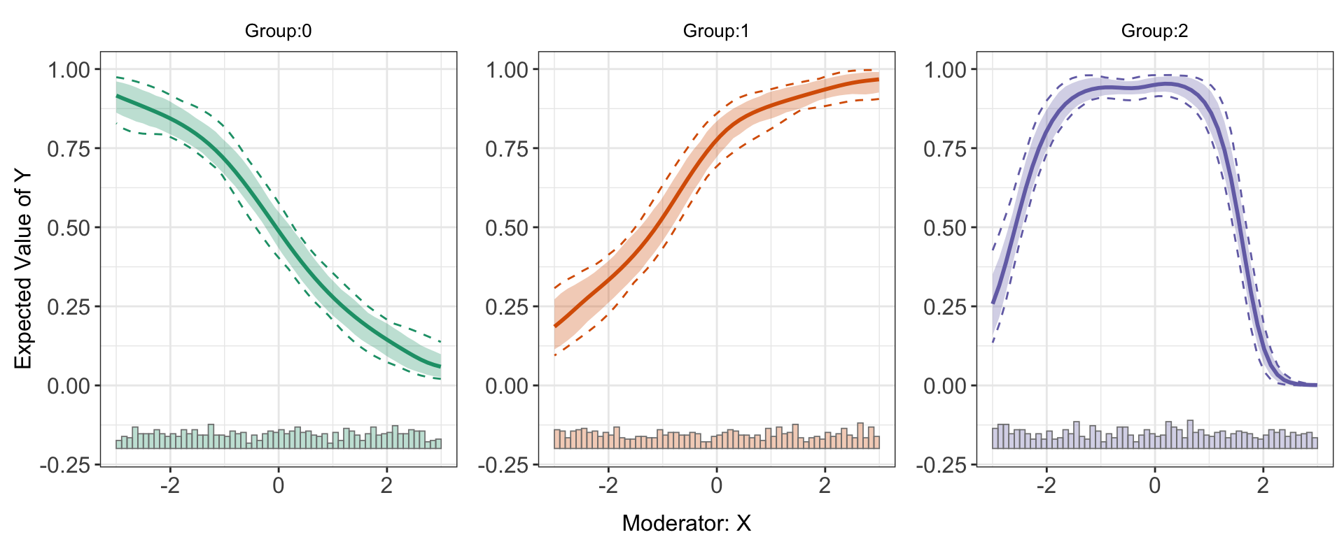
3.3 Predicted outcomes
As we have shown earlier with discrete outcome settings, interflex allows users to estimate and visualize predicted outcomes given fixed values of the treatment and moderator based on flexible interaction models. All predictions are made by setting covariates equal to their sample means. The same functino applies to continuous outcome as well.
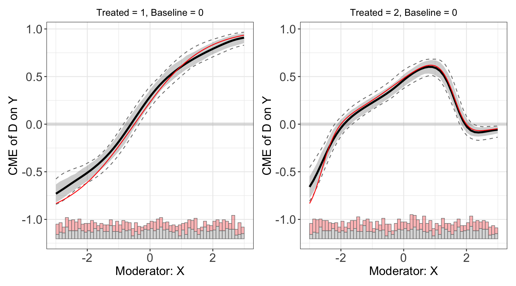
s5.kernel <-interflex(Y = "Y", D = "D", X = "X", Z = c("Z1", "Z2"),
                      data = s5, estimator = "kernel",vartype = 'bootstrap',
nboots = 200, parallel = TRUE, cores = 10)predict(s5.kernel)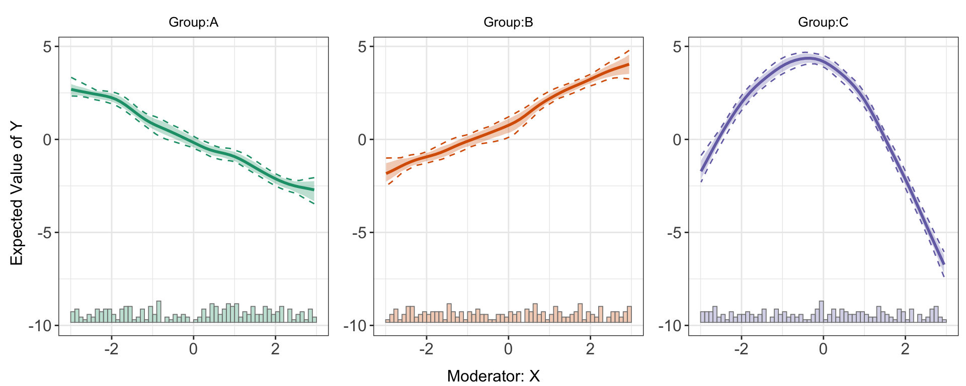
We can also use the linear model or the binning model to estimate and visualize predicted outcomes. For the latter, it is expected to see some “zigzags” at the bin boundaries in a plot:
s5.binning <-interflex(Y = "Y", D = "D", X = "X", Z = c("Z1","Z2"), data = s5,
estimator = "binning", vartype = "bootstrap", nbins = 4)predict(s5.binning)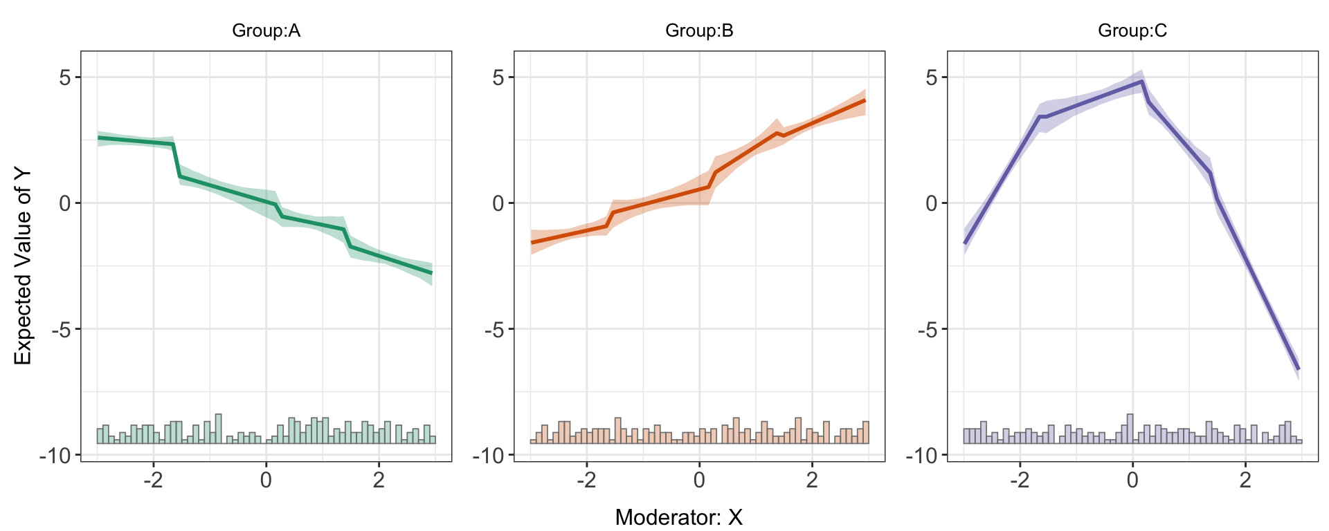
s5.linear <-interflex(Y = "Y", D = "D", X = "X", Z = c("Z1","Z2"),
                      data = s5,
estimator = "linear", vcov.type = "robust")predict(s5.linear)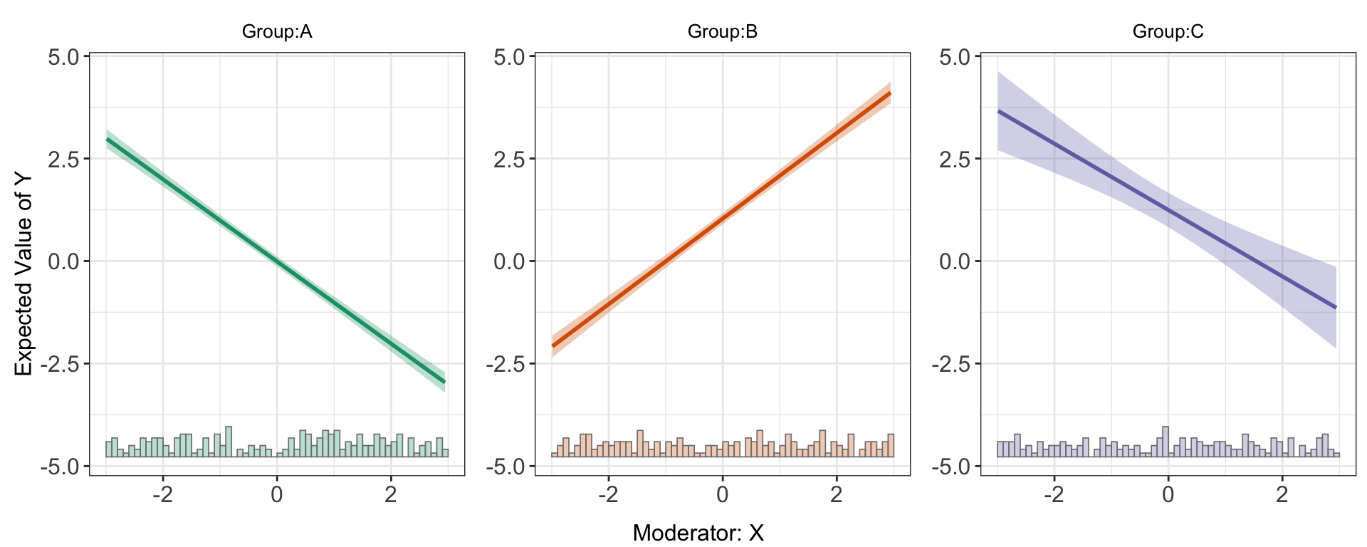
Obviously, the kernel estimator characterizes the data more better than a linear or binning estimator.
3.4 Effect modification
interflex allows users to estimate effect modification, i.e., by comparing treatment effects at three specific values of the moderator using linear or kernel model. In order to do so, users need to pass three values into diff.values when applying linear or kernel estimator. If not specified, this program will by default choose the 25,50,75 percentile of the moderator as the diff.values.
The difference of marginal effects/treatment effects at different values of the moderator(by default are the 25%, 50%, 75% quantiles of the moderator) are saved in diff.estimate.
s5.kernel$diff.estimate
#> $B
#>         diff.estimate    sd z-value p-value lower CI(95%) upper CI(95%)
#> 0 vs -2         4.109 0.280  14.659   0.000         3.564         4.684
#> 2 vs 0          4.427 0.298  14.850   0.000         3.851         4.935
#> 2 vs -2         8.536 0.235  36.389   0.000         8.109         9.009
#>
#> $C
#>         diff.estimate    sd z-value p-value lower CI(95%) upper CI(95%)
#> 0 vs -2         4.627 0.266  17.410   0.000         4.162         5.184
#> 2 vs 0         -4.385 0.278 -15.796   0.000        -4.896        -3.852
#> 2 vs -2         0.242 0.281   0.861   0.389        -0.267         0.744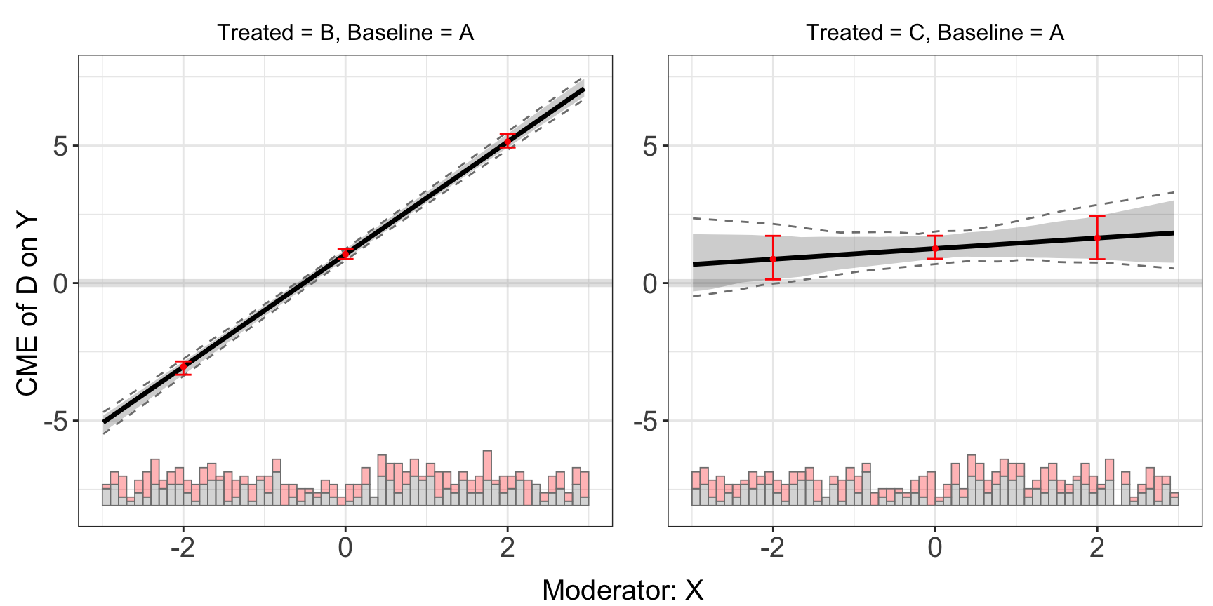
s5.linear$diff.estimate
#> $B
#>         diff.estimate    sd z-value p-value lower CI(95%) upper CI(95%)
#> 0 vs -2         4.090 0.094  43.615   0.000         3.922         4.278
#> 2 vs 0          4.090 0.094  43.615   0.000         3.922         4.278
#> 2 vs -2         8.179 0.188  43.615   0.000         7.845         8.555
#>
#> $C
#>         diff.estimate    sd z-value p-value lower CI(95%) upper CI(95%)
#> 0 vs -2         0.384 0.339   1.135   0.256        -0.259         1.042
#> 2 vs 0          0.384 0.339   1.135   0.256        -0.259         1.042
#> 2 vs -2         0.769 0.677   1.135   0.256        -0.518         2.084
interflex allows users to compare treatment effects at two or three specific values of the moderator using CME and vcov matrix derived from linear/kernel estimation. Based on GAM model(relies on mgcv package), users can approximate treatment effects and their variance using smooth functions without re-estimating the model, hence saving time. In order to do so, users need to pass the output of interflex into t.test and then specify the values of interest of the moderator. As it is an approximation, the results here are expected to have a little deviance from the output we got by directly specifying diff.values when applying inter.linear or inter.kernel. We also limit the elements passed in diff.values between the minimum and the maximum of the moderator to avoid potential extrapolation bias.
inter.test(s5.kernel,diff.values=c(-2,0,2))
#> $B
#>         diff.estimate    sd z-value p-value lower CI(95%) upper CI(95%)
#> 0 vs -2         4.101 0.279  14.721   0.000         3.555         4.647
#> 2 vs 0          4.429 0.296  14.964   0.000         3.849         5.009
#> 2 vs -2         8.530 0.234  36.375   0.000         8.070         8.989
#>
#> $C
#>         diff.estimate    sd z-value p-value lower CI(95%) upper CI(95%)
#> 0 vs -2         4.622 0.265  17.470   0.000         4.103         5.140
#> 2 vs 0         -4.386 0.276 -15.879   0.000        -4.927        -3.844
#> 2 vs -2 0.236 0.280 0.843 0.399 -0.313 0.785inter.test(s5.linear,diff.values=c(-2,0,2))
#> $B
#> diff.estimate sd z-value p-value lower CI(95%) upper CI(95%)
#> 0 vs -2 4.090 0.094 43.615 0.000 3.906 4.273
#> 2 vs 0 4.090 0.094 43.615 0.000 3.906 4.273
#> 2 vs -2 8.179 0.188 43.615 0.000 7.812 8.547
#>
#> $C
#> diff.estimate sd z-value p-value lower CI(95%) upper CI(95%)
#> 0 vs -2 0.384 0.339 1.135 0.256 -0.279 1.048
#> 2 vs 0 0.384 0.339 1.135 0.256 -0.279 1.048
#> 2 vs -2 0.769 0.677 1.135 0.256 -0.558 2.096We can also set percentile = TRUE to use the percentile scale rather than the real scale of the moderator.
inter.test(s5.kernel,diff.values=c(0.25,0.5,0.75),percentile=TRUE)
#> $B
#>            diff.estimate    sd z-value p-value lower CI(95%) upper CI(95%)
#> 50% vs 25%         3.040 0.282  10.769   0.000         2.487         3.593
#> 75% vs 50%         3.306 0.286  11.544   0.000         2.744         3.867
#> 75% vs 25%         6.346 0.264  24.076   0.000         5.829         6.862
#>
#> $C
#>            diff.estimate    sd z-value p-value lower CI(95%) upper CI(95%)
#> 50% vs 25%         2.811 0.287   9.795   0.000         2.249         3.374
#> 75% vs 50%        -2.647 0.274  -9.675   0.000        -3.183        -2.110
#> 75% vs 25%         0.165 0.309   0.533   0.594        -0.441         0.770
3.5 Discrete Moderator
In this section, we explore the special cases of CME where moderator \(X\) is discrete. When moderator \(X\) is discrete, the estimation of CME is a special case of estimating Conditional Average Treatment Effect (CATE), then marginalized over the moderator \(X\).
In the interflex package, we can estimate GATE with discrete moderator \(X\) using any estimator that supports gate = TRUE (e.g., linear, lasso, dml, grf). In the settings of binary treatment, the data is partitioned into groups based on moderator \(X\), and within each group the function estimates treatment effects separately.
We use empirical example from Beiser-McGrath and Bernauer (2024) to illustrate the implementation of interflex estimator with binary treatment.
data(app_bb2024)
#> Warning in data(app_bb2024): data set 'app_bb2024' not found
d<-app_bb2024
d<-remove_labels(d)

main<-"BB2024c6"
D="treat_type_bin"
Y="sup_tax_rebate"
X="income"

Z =c("leftright", "clim_belief", "resp_age", "female","employment_f", "highedu", "midedu", "pid_f")
Dlabel<-"Rebate"
Ylabel<-"Carbon Tax Support (with rebate)"
Xlabel<-"Income"
Visualization
out.raw <- interflex(estimator='raw', data = d,
                       Y = Y, D = D, X = X, Z = Z, na.rm = TRUE,
                       Ylabel = Ylabel, Dlabel = Dlabel,
                       Xlabel = Xlabel)
#> Baseline group not specified; choose treat = 0 as the baseline group.

out.raw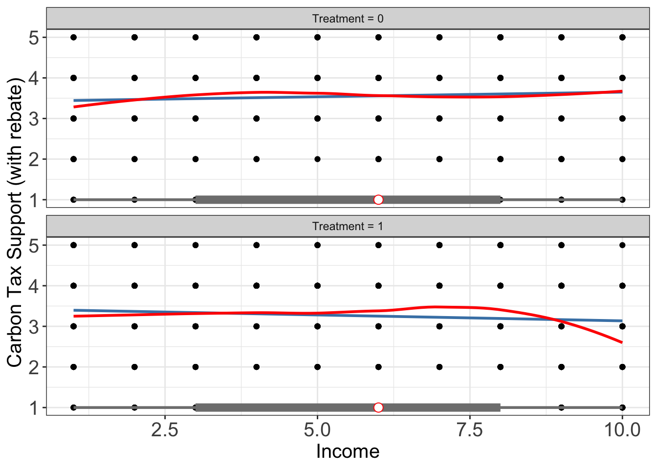
From the scatter plot, the treatment effect is positively correlated to moderator value \([5,8]\).
Estimation with kernel (treating X as continuous). We first estimate the CME using the kernel estimator without gate = TRUE, which treats the moderator as continuous and fits a smooth curve through the discrete X values:
out.kernel <- interflex(estimator='kernel', data = d,
                       Y = Y, D = D, X = X, Z = Z, na.rm = TRUE,
                       Ylabel = Ylabel, Dlabel = Dlabel,
                       Xlabel = Xlabel,
                       vartype = "bootstrap", nboots = 200)
#> Parallel computing: using 8 of 14 available cores.
#> To change: set cores = <n> in interflex().
#> Baseline group not specified; choose treat = 0 as the baseline group.
#> Cross-validating bandwidth ...
#> Optimal bw=4.0683.
#> Number of evaluation points:50out.kernel$figure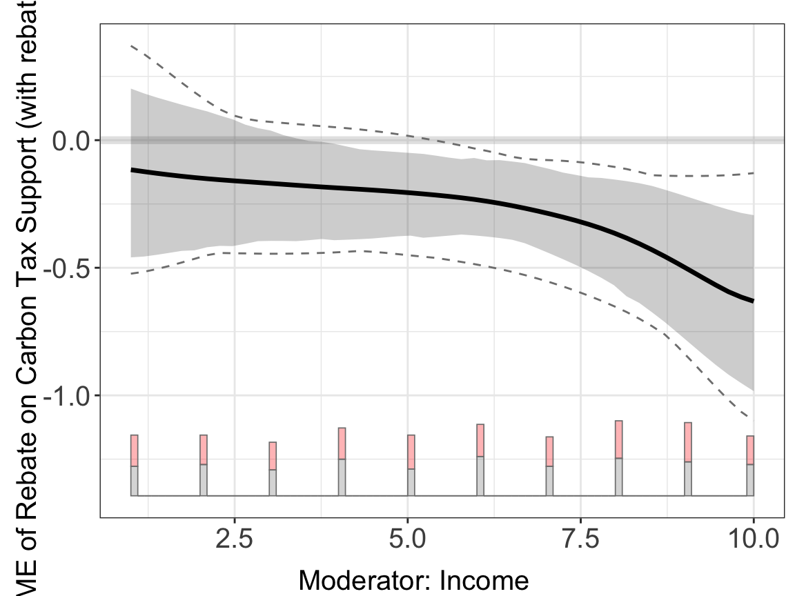
The smooth curve interpolates between discrete income levels, which may not be meaningful when the moderator is inherently categorical. A more natural approach is to evaluate the kernel regression only at the observed moderator values.
Estimation with kernel (gate = TRUE). Setting gate = TRUE tells interflex to evaluate the kernel estimator only at the observed discrete X levels, producing GATE point estimates:
out.kernel.gate <- interflex(estimator='kernel', data = d,
                       Y = Y, D = D, X = X, Z = Z, na.rm = TRUE,
                       Ylabel = Ylabel, Dlabel = Dlabel,
                       Xlabel = Xlabel,
                       vartype = "bootstrap", nboots = 200,
                       gate = TRUE)
#> Parallel computing: using 8 of 14 available cores.
#> To change: set cores = <n> in interflex().
#> Baseline group not specified; choose treat = 0 as the baseline group.
#> Cross-validating bandwidth ...
#> Optimal bw=6.5511.
#> Number of evaluation points:10out.kernel.gate$figure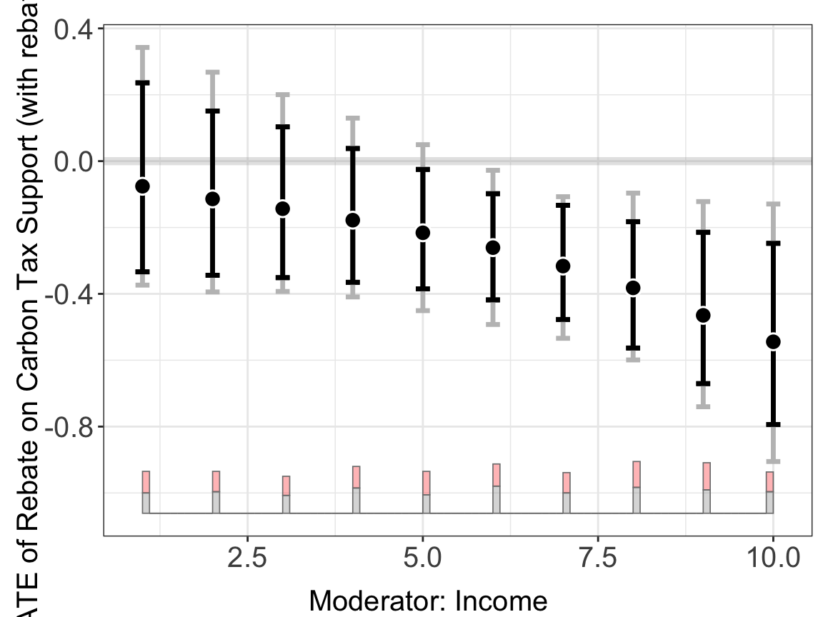
When gate = TRUE, the plot automatically shows separate point estimates and confidence intervals for each discrete level of the moderator, rather than a smooth curve.