data(app_et2023)
#> Warning in data(app_et2023): data set 'app_et2023' not found
d<-app_et2023
d<-remove_labels(d)

main<-"Egerod & Tran 2023"
D="did"
Y="seats_t_ind"
X="abs_nom"

Z = c("sen", "hloga")
# Dlabel<-"Honest Leadership and Open Government Ac"
Dlabel<-"Treatment"
# Ylabel<-"ATT of HLOGA on Board Service"
Ylabel<-"Outcome"
Xlabel<-"Ideological Extremism"
cl <- "state_po"6 Discrete outcome
Discrete outcomes require different modeling strategies with link functions, thus change how we implement and interpret CME estimation. In interflex package, we provide four options for link function: method = "probit" or "logit", "poisson", "nbinom"; In the package, probit and logit support binary outcome, poisson and nbinom support outcome with count distributions.
Example: Egerod and Tran (2023)
6.0.1 Classic approach
6.0.1.1 Binning estimator
The binning estimator is a diagnostic tool, it will discretizes the moderator \(X\) into several bins and create a dummy variable for each bin and picks an evaluation point within each bin, where users want to estimate the conditional marginal effect (CME) of \(D\) on \(Y\). The regression terms includes interactions between the bin dummies and the treatment indicator, the bin dummies and the moderator \(X\) minus the evaluation points, as well as the triple interactions.
Estimation.
out.binning <- interflex(estimator='binning', method='logit', data = d,
                       Y = Y, D = D, X = X, Z = Z, na.rm = TRUE,
                       Ylabel = Ylabel, Dlabel = Dlabel,
                       Xlabel = Xlabel)
#> Baseline group not specified; choose treat = 0 as the baseline group.out.binning$figure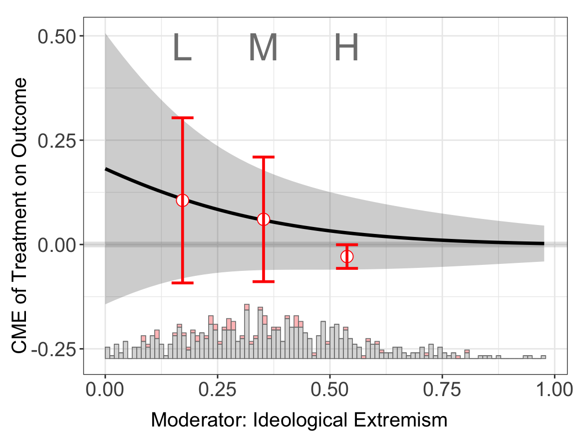
If the CME estimates from the binning estimator sit closely to the estimated CME from the linear estimator, then the LIE assumption likely holds. For this example, it is clear that first two binning estimators sits closely to the results from linear estimator.
The program provides formal tools for verifying the the LIE assumption, the Wald test and the likelihood ratio test. For , both of these two tests reject the null hypothesis of LIE.
Results. The CME plot is stored in $figure while the estimates and standard errors are stored in $est.lin.
head(out.binning$est.bin[[1]])
#>                                               x0        coef         sd
#> Ideological Extremism:[3.58e-10,0.272] 0.1720000  0.10572933 0.10071644
#> Ideological Extremism:(0.272,0.432]    0.3522321  0.06027958 0.07600450
#> Ideological Extremism:(0.432,0.977]    0.5379063 -0.02886648 0.01443028
#>                                           CI.lower     CI.upper
#> Ideological Extremism:[3.58e-10,0.272] -0.09211552  0.303574174
#> Ideological Extremism:(0.272,0.432]    -0.08902176  0.209580921
#> Ideological Extremism:(0.432,0.977]    -0.05721297 -0.000519996
One can visualize \(E(Y|X,D,Z)\) estimated using the binning model. It is expected to see some “zigzags” at the bin boundaries in the plot.
predict(out.binning)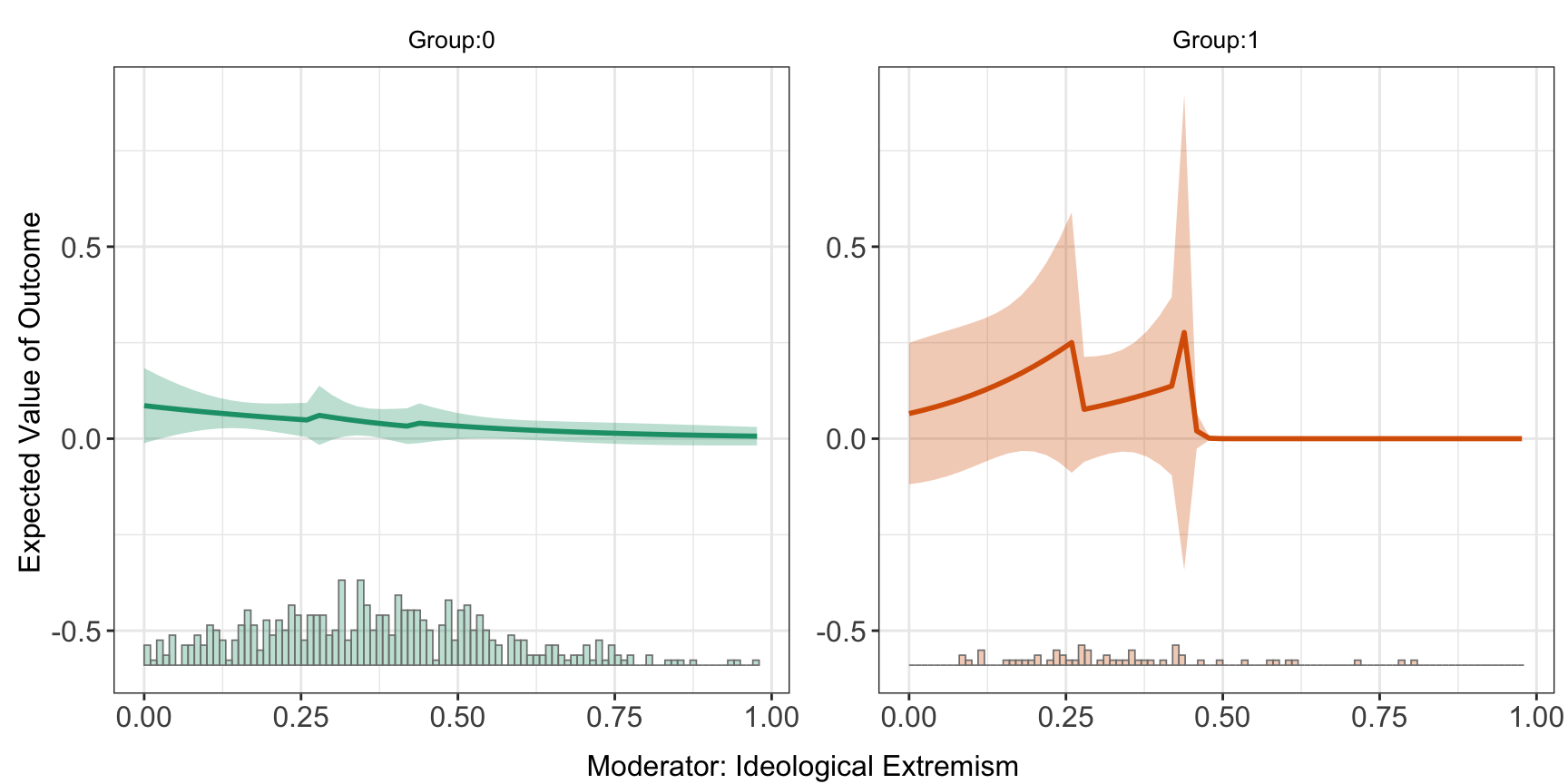
6.0.1.2 Linear estimator
Estimations. When setting the option estimator to linear, the program will conduct the classic glm regression and estimate the CME using the coefficients from the regression. In the following command, the outcome variable is \(Y\), the moderator is \(X\), the covariates is \(Z\), and here it uses logit link function.
out.linear.1 <- interflex(estimator='linear', method='logit', data = d,
                       Y = Y, D = D, X = X, Z = Z, na.rm = TRUE,
                       Ylabel = Ylabel, Dlabel = Dlabel,
                       Xlabel = Xlabel)
#> Baseline group not specified; choose treat = 0 as the baseline group.out.linear.1$figure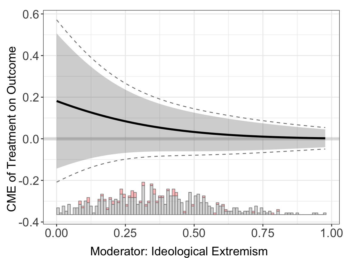
For the linear estimator, when the option full.moderate is set to TRUE, interaction terms between the moderator \(X\) and each covariate will enter the model, which is the case in Blackwell and Olson (2022). This extension in some cases can reduce the bias of the original model.
User can also specify different link function by changing the method option.
out.linear.2 <- interflex(estimator='linear', method='logit', data = d,
                       Y = Y, D = D, X = X, Z = Z, na.rm = TRUE,
                       Ylabel = Ylabel, Dlabel = Dlabel,
                       Xlabel = Xlabel, ylim = c(-0.4,0.6))
#> Baseline group not specified; choose treat = 0 as the baseline group.

out.linear.3 <- interflex(estimator='linear', method='probit', data = d,
                       Y = Y, D = D, X = X, Z = Z, na.rm = TRUE,
                       Ylabel = Ylabel, Dlabel = Dlabel,
                       Xlabel = Xlabel, ylim = c(-0.4,0.6))
#> Baseline group not specified; choose treat = 0 as the baseline group.

out.linear.4 <- interflex(estimator='linear', method='logit', data = d,
                       Y = Y, D = D, X = X, Z = Z, na.rm = TRUE,
                       Ylabel = Ylabel, Dlabel = Dlabel,
                       full.moderate = TRUE,
                       Xlabel = Xlabel, ylim = c(-0.4,0.6))
#> Use fully moderated model.
#> Baseline group not specified; choose treat = 0 as the baseline group.ggarrange(out.linear.2$figure, out.linear.3$figure, out.linear.4$figure,
ncol = 3)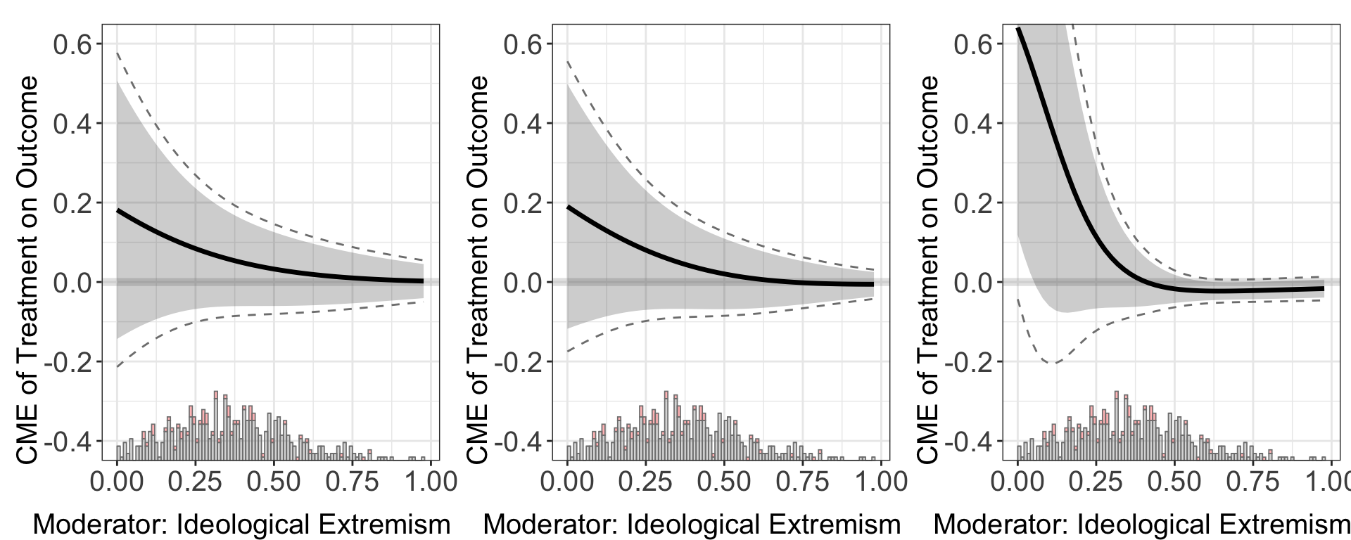
Continuous treatment. As the CME in glm models also depends on the value of \(D\), users can pass their preferred values of \(D\) into the option D.ref.
Uncertainty estimation. In the default setting, confidence intervals of CME are estimated using the delta method. The program also supports the bootstrap method and the simulation methods simu. Noted that uniform CI is not available for vartype = simu.
out.linear.2 <- interflex(estimator='linear', method='logit', data = d,
                       Y = Y, D = D, X = X, Z = Z, na.rm = TRUE,
                       Ylabel = Ylabel, Dlabel = Dlabel, vartype = "delta",
                       Xlabel = Xlabel, ylim = c(-0.4,0.6))
#> Baseline group not specified; choose treat = 0 as the baseline group.

out.linear.3 <- interflex(estimator='linear', method='probit', data = d,
                       Y = Y, D = D, X = X, Z = Z, na.rm = TRUE,
                       Ylabel = Ylabel, Dlabel = Dlabel, vartype = "bootstrap",
                       Xlabel = Xlabel, ylim = c(-0.4,0.6))
#> Parallel computing: using 8 of 14 available cores.
#> To change: set cores = <n> in interflex().
#> Baseline group not specified; choose treat = 0 as the baseline group.
#> Note: Insufficient bootstrap samples (B=200) for Bootstrapped Uniform CI with 50 evaluation points. Using Bonferroni CI by default. Consider increasing nboots for tighter uniform bands.

out.linear.4 <- interflex(estimator='linear', method='logit', data = d,
                       Y = Y, D = D, X = X, Z = Z, na.rm = TRUE,
                       Ylabel = Ylabel, Dlabel = Dlabel, vartype = "simu",
                       Xlabel = Xlabel, ylim = c(-0.4,0.6))
#> Baseline group not specified; choose treat = 0 as the baseline group.ggarrange(out.linear.2$figure, out.linear.3$figure, out.linear.4$figure,
ncol = 3)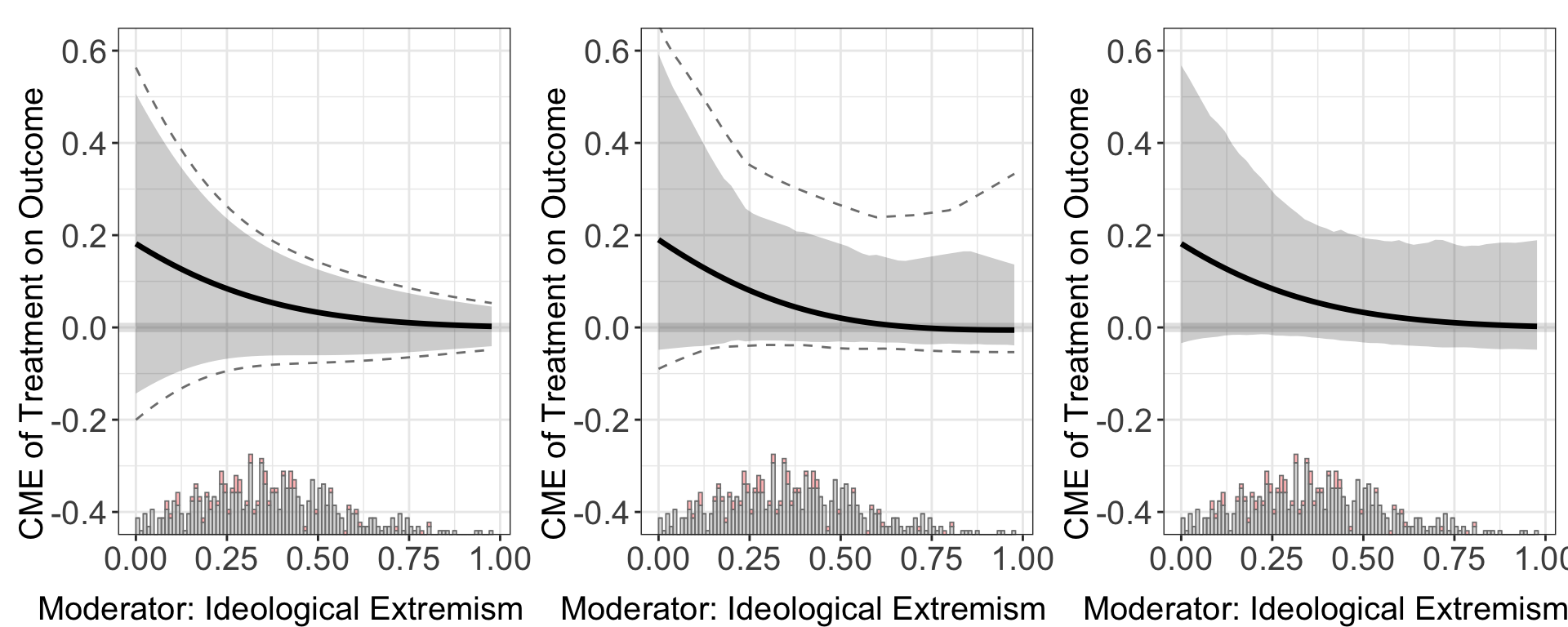
Results. The CME plot is stored in out$figure while the estimates and standard errors are stored in out$est.lin.
head(out.linear.1$est.lin$`1`)
#>                 X        ME        sd lower CI(95%) upper CI(95%)
#> [1,] 3.576279e-10 0.1815824 0.1653932    -0.1433012     0.5064660
#> [2,] 1.993282e-02 0.1719692 0.1557089    -0.1338915     0.4778298
#> [3,] 3.986565e-02 0.1626554 0.1464285    -0.1249756     0.4502865
#> [4,] 5.979847e-02 0.1536517 0.1375831    -0.1166041     0.4239075
#> [5,] 7.973129e-02 0.1449662 0.1291973    -0.1088174     0.3987498
#> [6,] 9.966411e-02 0.1366048 0.1212898    -0.1016460     0.3748557
#>      lower uniform CI(95%) upper uniform CI(95%)
#> [1,]            -0.2085735             0.5717383
#> [2,]            -0.1953418             0.5392802
#> [3,]            -0.1827635             0.5080743
#> [4,]            -0.1709011             0.4782045
#> [5,]            -0.1598050             0.4497374
#> [6,]            -0.1495129             0.4227226
The estimated \(E[Y |X, Z,D]\) are saved in. User can specify either 1 for treatment group, or 0 for control group.
head(out.linear.1$pred.lin$`1`)
#>                 X      E(Y)        sd lower CI(95%) upper CI(95%)
#> [1,] 3.576279e-10 0.2687853 0.1658573   -0.05700985     0.5945804
#> [2,] 1.993282e-02 0.2557372 0.1560203   -0.05073505     0.5622094
#> [3,] 3.986565e-02 0.2431119 0.1465628   -0.04478289     0.5310067
#> [4,] 5.979847e-02 0.2309166 0.1375182   -0.03921194     0.5010451
#> [5,] 7.973129e-02 0.2191558 0.1289137   -0.03407078     0.4723824
#> [6,] 9.966411e-02 0.2078322 0.1207702   -0.02939799     0.4450624
The estimated average treatment effect (ATE) is saved in Avg.estimate. Here the program uses the coefficients from the regression and the input data to calculate the ATE/AME.
head(out.linear.1$Avg.estimate)
#> $`1`
#>                            ATE    sd z-value p-value lower CI(95%)
#> Average Treatment Effect 0.129 0.100   1.291   0.197        -0.067
#>                          upper CI(95%)
#> Average Treatment Effect         0.325
The estimated difference of treatment effects are saved in diff.estimate:
head(out.linear.1$diff.estimate)
#> $`1`
#>            diff.estimate    sd z-value p-value lower CI(95%) upper CI(95%)
#> 50% vs 25%        -0.031 0.032  -0.981   0.326        -0.093         0.031
#> 75% vs 50%        -0.024 0.022  -1.090   0.276        -0.067         0.019
#> 75% vs 25%        -0.055 0.053  -1.034   0.301        -0.160         0.050
6.0.1.3 Kernel estimator
Estimation.
out.kernel <- interflex(estimator='kernel', method='logit', data = d,
                       Y = Y, D = D, X = X, Z = Z, na.rm = TRUE,
                       Ylabel = Ylabel, Dlabel = Dlabel,
                       vartype = "bootstrap", ylim = c(-0.4, 0.6),
                       Xlabel = Xlabel)
#> Parallel computing: using 8 of 14 available cores.
#> To change: set cores = <n> in interflex().
#> Baseline group not specified; choose treat = 0 as the baseline group.
#> Cross-validating bandwidth ...
#> Optimal bw=0.6066.
#> Number of evaluation points:50out.kernel$figure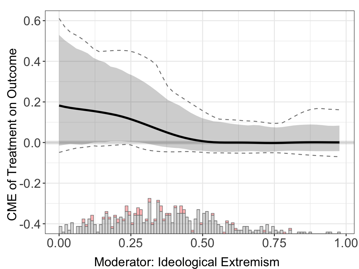
Uncertainty estimation. With the kernel method, a bandwidth is first selected via a 10-fold cross-validation. If the outcome variable is binary, the bandwidth that produces the largest area under the curve (AUC) or the least cross entropy in cross validation will be chosen as the “optimal” bandwidth. The standard errors are produced by a non-parametric bootstrap. It is very flexible but takes more time compared with the linear estimation. The nboots, bw, and grid option for choosing bandwidths is also available in discrete outcome settings.
Results. The estimation results, including pointwise and uniform confidence intervals, are included in est.kernel.
head(out.kernel$est.kernel$`1`)
#>                 X        TE        sd lower CI(95%) upper CI(95%)
#> [1,] 3.576279e-10 0.1820826 0.1546284  -0.015388873     0.5298434
#> [2,] 1.993282e-02 0.1756441 0.1486050  -0.010732080     0.5033522
#> [3,] 3.986565e-02 0.1705892 0.1428735  -0.006878991     0.4834832
#> [4,] 5.979847e-02 0.1664770 0.1372925  -0.008819091     0.4631741
#> [5,] 7.973129e-02 0.1627995 0.1318920  -0.010497129     0.4523927
#> [6,] 9.966411e-02 0.1591086 0.1265307  -0.006164256     0.4392779
#>      lower uniform CI(95%) upper uniform CI(95%)
#> [1,]           -0.04869196             0.6111846
#> [2,]           -0.04104702             0.5694517
#> [3,]           -0.03394524             0.5422840
#> [4,]           -0.02755963             0.5283411
#> [5,]           -0.02455510             0.5106260
#> [6,]           -0.02126167             0.4884395
The results of cross-validation are saved in CV.output.
head(out.kernel$CV.output)
#>               bw Num.Eff.Points Cross Entropy       AUC        MSE        MAE
#> [1,] 0.009767083           46.7      2.090611 0.6509684 0.09205258 0.10111807
#> [2,] 0.011448021           46.2      1.864904 0.6149909 0.08474748 0.09637160
#> [3,] 0.013418251           46.7      1.641831 0.5475765 0.08210697 0.09647201
#> [4,] 0.015727563           47.4      1.610359 0.5575096 0.08785981 0.10655850
#> [5,] 0.018434313           46.7      1.447244 0.6976763 0.08393787 0.10758211
#> [6,] 0.021606901           48.0      1.316970 0.6636500 0.08426880 0.11287031
Like the linear estimator, the estimated conditional effects \(E[Y | X, D, Z]\) is saved in “pred.kernel”. Users can visualize it using the command “predict”.
head(out.kernel$pred.kernel$`1`)
#>                 X      E(Y)        sd lower CI(95%) upper CI(95%)
#> [1,] 3.576279e-10 0.2631406 0.1544828    0.08402310     0.5933896
#> [2,] 1.993282e-02 0.2523193 0.1483467    0.08099363     0.5666793
#> [3,] 3.986565e-02 0.2434197 0.1424896    0.07836495     0.5472697
#> [4,] 5.979847e-02 0.2359783 0.1368179    0.07553569     0.5265371
#> [5,] 7.973129e-02 0.2294243 0.1313451    0.07208620     0.5094576
#> [6,] 9.966411e-02 0.2232272 0.1259219    0.06828006     0.4989420
#>      lower uniform CI(95%) upper uniform CI(95%)
#> [1,]            0.04613839             0.6526999
#> [2,]            0.04486173             0.6281901
#> [3,]            0.04435149             0.6051091
#> [4,]            0.04468932             0.5879602
#> [5,]            0.04583041             0.5676422
#> [6,]            0.04755542             0.5434046
predict(out.kernel)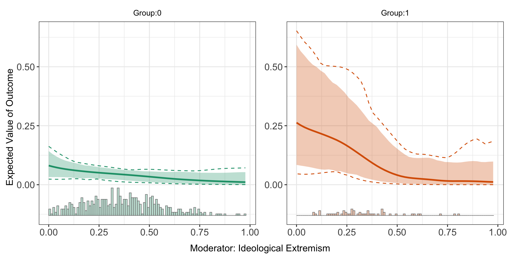
The estimated average treatment effect (ATE) is saved in Avg.estimate, and the estimated difference of treatment effects are saved in diff.estimate:
head(out.kernel$Avg.estimate)
#> $`1`
#>                            ATE    sd z-value p-value lower CI(95%)
#> Average Treatment Effect 0.131 0.080   1.624   0.104        -0.043
#>                          upper CI(95%)
#> Average Treatment Effect         0.269
head(out.kernel$diff.estimate)
#> $`1`
#>            diff.estimate    sd z-value p-value lower CI(95%) upper CI(95%)
#> 50% vs 25%        -0.061 0.048  -1.267   0.205        -0.175         0.014
#> 75% vs 50%        -0.052 0.036  -1.440   0.150        -0.151        -0.008
#> 75% vs 25%        -0.113 0.077  -1.470   0.142        -0.284        -0.002
6.0.2 Lasso approach
Traditional parametric approaches for binary or count data typically rely on link functions - such as logit, probit, poisson, or negative binomial - to capture nonlinearity between predictors and the outcome. However, this introduces two key challenges. First, it becomes difficult to disentangle the nonlinearity imposed by the link function from the intrinsic nonlinearity of the CME. Second, when the treatment (D) is continuous, the derivative \((\frac{\partial Y}{\partial D})\) depends on both (X) and (D), requiring an additional averaging over (D) to recover a coherent measure of the CME: \((\mathbb{E}\left[\left.\frac{\partial Y}{\partial D}\right\rvert X = x\right])\).
When the treatment is binary, the link function can be naturally incorporated into the Lasso estimator by modifying the learner to model the outcome appropriately. When the treatment is continuous, although the theoretical framework underlying the PO-Lasso is based on the partially linear regression model - which does not explicitly account for the link function - these methods can still serve as good approximations.
To estimate CME with discrete outcome using Lasso-based estimator, the syntax is exactly the same with continuous treatment settings, so we don’t need to spcify the link function.
out.lasso <- interflex(estimator='lasso', data = d,
                       Y = Y, D = D, X = X, Z = Z, na.rm = TRUE,
                       Ylabel = Ylabel, Dlabel = Dlabel,
                       vartype = "bootstrap", ylim = c(-0.4, 0.6),
                       Xlabel = Xlabel)
#> Parallel computing: using 8 of 14 available cores.
#> To change: set cores = <n> in interflex().
#> Baseline group not specified; choose treat = 0 as the baseline group.
#> >> Treatment is binary/discrete.
#>    Signal = aipw
#>    Estimand = ATE
#>    Basis extension = bspline
#>    Outcome model = lasso; PS model = lasso
#> Step 1: Matching arguments and setting defaults...
#> Step 2: Performing basic checks on input data...
#> Step 3: Processing fixed effects (if provided)...
#> Step 4: Setting up evaluation grid for X (if not provided)...
#> Step 5: Building design matrix...
#> Design matrix successfully built.
#> Step 6: Setting up model types based on signal argument...
#> Step 7: Fitting outcome and propensity score models...
#>    Fitting outcome model for treated (D=1) units...
#>    Fitting propensity score model (no FE)...
#> Step 8: Performing post-lasso variable selection (if applicable)...
#>    Post-lasso: refitting outcome and propensity score models on selected variables...
#> Step 9: Generating predictions from fitted models...
#> Step 10: Computing signals and performing dimension reduction...
#> Step 11: Estimation complete. Returning results.out.lasso$figure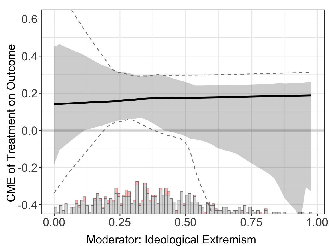
Because the sample size is small (\(n = 570\)), the AIPW estimator doesn’t perform very well.
6.0.3 Double machine learning
Similar to the Lasso estimator, when treatment is binary the link function can be naturally incorporated into the DML estimator as well. When the treatment is continuous, DML estimator can serve as good approximations via the partially linear regression model.
To estimate CME with discrete outcome using DML estimator, the syntax is the same with both binary and continuous treatment settings:
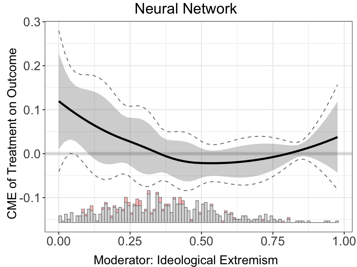
binary.dml.nn.nn <- interflex(estimator="dml", data = d,
                              Y = Y, D = D, X = X, Z = Z, na.rm = TRUE,
                              Ylabel = Ylabel, Dlabel = Dlabel,
                              Xlabel = Xlabel,
                              model.y = "nn", model.t = "nn",
                              main = "Neural Network")
#> Parallel computing: using 8 of 14 available cores.
#> To change: set cores = <n> in interflex().
#> Baseline group not specified; choose treat = 0 as the baseline group.binary.dml.nn.nn$figure