library(interflex)
data(interflex)
ls()
#>  [1] "app_adiguzel2023" "app_bb2024"       "app_et2023"       "app_hma2015"
#>  [5] "app_vernby2013"   "packages"         "pkg"              "s1"
#>  [9] "s2"               "s3"               "s4"               "s5"
#> [13] "s6"               "s7"               "s8"               "s9"

d<-app_hma2015

## Define variables
Y = "totangry" ## outcome: anger
D = "threat" ## treatment: threat
X = "pidentity" ## moderator: partisan identity
Z <-  c("issuestr2", "knowledge", "educ","male", "age10")

Ylabel = "Anger"
Dlabel = "Threat"
Xlabel = "Partisanship"4 Lasso Methods
In this chapter, we introduce Lasso-based approaches for estimating the conditional marginal effect (CME), addressing limitations of traditional outcome-modeling methods. When the treatment is binary, we use Lasso within an augmented inverse probability weighting (AIPW) framework. This approach integrates both the outcome model and the propensity score model, yielding a doubly robust estimator that remains consistent as long as at least one of the two models is correctly specified. When the treatment is continuous, we employ a “partial-out” (PO) estimator: Lasso is used to denoise both the outcome and treatment variables with respect to covariates (or potential fixed effects), and a kernel method is then applied to the denoised variables to estimate the conditional marginal effect.
4.1 Binary treatment
The Lasso framework for estimating CME follows a three‐step procedure: (1) model the outcome and the propensity score; (2) construct signals; and (3) smooth the signals over the moderator \(X\). In the first step, one can perform a basis expansion and include interaction terms to account for potential nonlinearity and interaction effects among covariates.
When the number of covariates or their expanded basis functions is large, conventional OLS or logistic regression may overfit and yield unstable estimates. In the interflex package, we use post‐selection Lasso for feature selection to ensure valid standard errors. In this user manual, we refer to the AIPW estimator with basis expansion and post‐Lasso selection as AIPW‐Lasso: we first use Lasso regression for feature selection, then run a post‐Lasso OLS regression to obtain the coefficients for those selected features. In the next step, we construct the AIPW signal to ensure double robustness; in the final step, we apply a kernel regression to smooth the signals over the moderator \(X\).
In the binary‐treatment setting, we use the Huddy et al. (2015) example, where the outcome variable is the level of anger, the treatment variable indicates an electoral loss threat or an electoral win reassurance, and the moderator \(X\) represents the strength of partisan identity.
4.1.0.1 AIPW-Lasso estimator
Estimation. To estimate the CME with the AIPW‐Lasso estimator, set the option estimator = "lasso".
Uncertainty estimation. The standard error of the AIPW‐Lasso estimator is calculated via nonparametric bootstrapping. The default number of bootstrap samples, nboots, is 200—you can increase nboots for more stable standard‐error estimates. Both pointwise and uniform confidence intervals are provided in the plot.
Results. The estimation results are stored in est.aipw, which includes the corresponding \(X\) values, point estimates, standard errors, and lower/upper bounds for both uniform and pointwise confidence intervals.
aipw.out.1 <- interflex(estimator = "lasso", data = d,
                 Y = Y,D = D, X = X, Z = Z,
                 Ylabel = Ylabel, Dlabel = Dlabel,
                 Xlabel = Xlabel,
                 main = "AIPW-Lasso estimation")
#> Parallel computing: using 8 of 14 available cores.
#> To change: set cores = <n> in interflex().
#> Baseline group not specified; choose treat = 0 as the baseline group.
#> >> Treatment is binary/discrete.
#>    Signal = aipw
#>    Estimand = ATE
#>    Basis extension = bspline
#>    Outcome model = lasso; PS model = lasso
#> Step 1: Matching arguments and setting defaults...
#> Step 2: Performing basic checks on input data...
#> Step 3: Processing fixed effects (if provided)...
#> Step 4: Setting up evaluation grid for X (if not provided)...
#> Step 5: Building design matrix...
#> Design matrix successfully built.
#> Step 6: Setting up model types based on signal argument...
#> Step 7: Fitting outcome and propensity score models...
#>    Fitting outcome model for treated (D=1) units...
#>    Fitting propensity score model (no FE)...
#> Step 8: Performing post-lasso variable selection (if applicable)...
#>    Post-lasso: refitting outcome and propensity score models on selected variables...
#> Step 9: Generating predictions from fitted models...
#> Step 10: Computing signals and performing dimension reduction...
#> Step 11: Estimation complete. Returning results.aipw.out.1$figure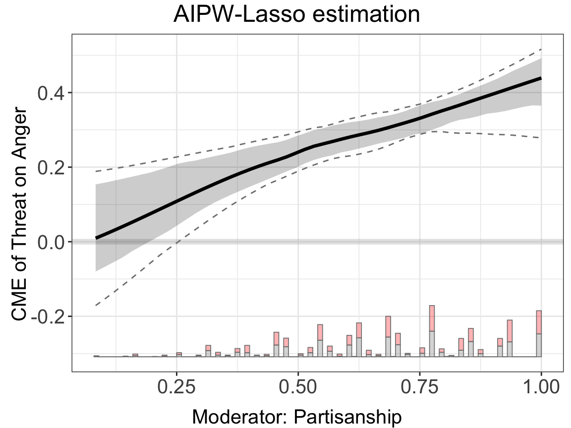
head(aipw.out.1$est.lasso[[1]])
#>            X         CME         SE    CI.lower  CI.upper CI.lower.uniform
#> 1 0.08333334 0.009371894 0.06518669 -0.07993894 0.1537738      -0.17114686
#> 2 0.10204082 0.019618878 0.06274102 -0.06741399 0.1583518      -0.15364193
#> 3 0.12074830 0.030207643 0.06023282 -0.05457476 0.1636376      -0.13540290
#> 4 0.13945578 0.041085516 0.05768253 -0.04146929 0.1689829      -0.11654217
#> 5 0.15816327 0.052199820 0.05432956 -0.02540226 0.1743585      -0.09717212
#> 6 0.17687075 0.063497880 0.05181190 -0.01189882 0.1800390      -0.07740513
#>   CI.upper.uniform
#> 1        0.1885818
#> 2        0.1920907
#> 3        0.1959243
#> 4        0.2000328
#> 5        0.2043665
#> 6        0.2088754
4.1.0.2 Advance options
In AIPW-Lasso estimator, we provide several advanced options, allowing greater flexibility for user to deploy the estimator.
4.1.0.2.1 Signals
Signals refer to transformations of the data that are relevant for the target‐parameter estimation, as commonly used in the double‐robustness literature. We provide three options for the signal parameter in the AIPW‐Lasso estimator: outcome, ipw, and aipw (default).
When the signal is set to ipw, we are effectively estimating the CME with an IPW estimator, which can be sensitive to extreme weights, particularly when the estimated propensity score is close to 0 or 1.
aipw.out.outcome <- interflex(estimator = "lasso", data = d,
                 Y = Y,D = D, X = X, Z = Z,
                 Ylabel = Ylabel, Dlabel = Dlabel,
                 Xlabel = Xlabel, nboots = 200, signal = "outcome",
                 main = "Signal: outcome")
#> Parallel computing: using 8 of 14 available cores.
#> To change: set cores = <n> in interflex().
#> Baseline group not specified; choose treat = 0 as the baseline group.
#> >> Treatment is binary/discrete.
#>    Signal = outcome
#>    Estimand = ATE
#>    Basis extension = bspline
#>    Outcome model = lasso; PS model = lasso
#> Step 1: Matching arguments and setting defaults...
#> Step 2: Performing basic checks on input data...
#> Step 3: Processing fixed effects (if provided)...
#> Step 4: Setting up evaluation grid for X (if not provided)...
#> Step 5: Building design matrix...
#> Design matrix successfully built.
#> Step 6: Setting up model types based on signal argument...
#> Step 7: Fitting outcome and propensity score models...
#>    Fitting outcome model for treated (D=1) units...
#> Step 8: Performing post-lasso variable selection (if applicable)...
#>    Post-lasso: refitting outcome models on selected variables...
#> Step 9: Generating predictions from fitted models...
#> Step 10: Computing signals and performing dimension reduction...
#> Step 11: Estimation complete. Returning results.

aipw.out.ipw <- interflex(estimator = "lasso", data = d,
                 Y = Y,D = D, X = X, Z = Z,
                 Ylabel = Ylabel, Dlabel = Dlabel,
                 Xlabel = Xlabel, signal = "ipw",
                 main = "Signal: IPW")
#> Parallel computing: using 8 of 14 available cores.
#> To change: set cores = <n> in interflex().
#> Baseline group not specified; choose treat = 0 as the baseline group.
#> >> Treatment is binary/discrete.
#>    Signal = ipw
#>    Estimand = ATE
#>    Basis extension = bspline
#>    Outcome model = lasso; PS model = lasso
#> Step 1: Matching arguments and setting defaults...
#> Step 2: Performing basic checks on input data...
#> Step 3: Processing fixed effects (if provided)...
#> Step 4: Setting up evaluation grid for X (if not provided)...
#> Step 5: Building design matrix...
#> Design matrix successfully built.
#> Step 6: Setting up model types based on signal argument...
#> Step 7: Fitting outcome and propensity score models...
#>    Fitting propensity score model (no FE)...
#> Step 8: Performing post-lasso variable selection (if applicable)...
#> Step 9: Generating predictions from fitted models...
#> Step 10: Computing signals and performing dimension reduction...
#> Step 11: Estimation complete. Returning results.

aipw.out.aipw <- interflex(estimator = "lasso", data = d,
                 Y = Y,D = D, X = X, Z = Z,
                 Ylabel = Ylabel, Dlabel = Dlabel,
                 Xlabel = Xlabel, signal = "aipw",
                 main = "Signal: AIPW")
#> Parallel computing: using 8 of 14 available cores.
#> To change: set cores = <n> in interflex().
#> Baseline group not specified; choose treat = 0 as the baseline group.
#> >> Treatment is binary/discrete.
#>    Signal = aipw
#>    Estimand = ATE
#>    Basis extension = bspline
#>    Outcome model = lasso; PS model = lasso
#> Step 1: Matching arguments and setting defaults...
#> Step 2: Performing basic checks on input data...
#> Step 3: Processing fixed effects (if provided)...
#> Step 4: Setting up evaluation grid for X (if not provided)...
#> Step 5: Building design matrix...
#> Design matrix successfully built.
#> Step 6: Setting up model types based on signal argument...
#> Step 7: Fitting outcome and propensity score models...
#>    Fitting outcome model for treated (D=1) units...
#>    Fitting propensity score model (no FE)...
#> Step 8: Performing post-lasso variable selection (if applicable)...
#>    Post-lasso: refitting outcome and propensity score models on selected variables...
#> Step 9: Generating predictions from fitted models...
#> Step 10: Computing signals and performing dimension reduction...
#> Step 11: Estimation complete. Returning results.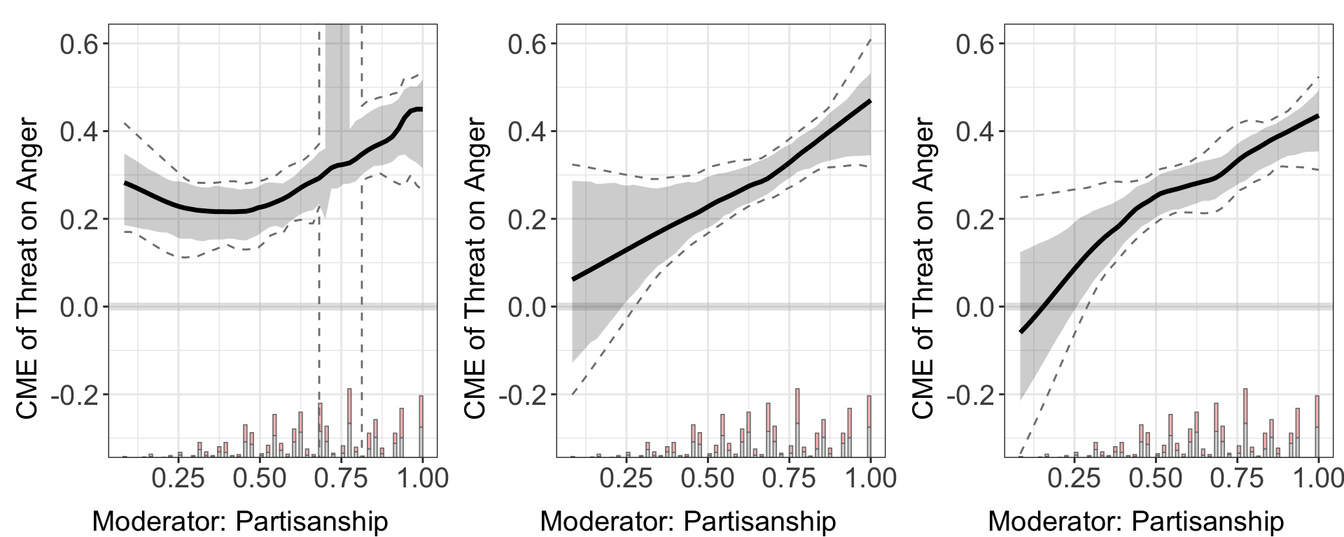
4.1.0.2.2 ATE vs ATT
With a binary treatment, we can also set the estimand to the average treatment effect on the treated (ATT) rather than the average treatment effect (ATE) (default). We can use the estimand option for this purpose. It also supports the outcome, ipw, and aipw (default) signals.
aipw.out.ate <- interflex(estimator = "lasso", data = d,
                 Y = Y,D = D, X = X, Z = Z,
                 Ylabel = Ylabel, Dlabel = Dlabel,
                 Xlabel = Xlabel,
                 estimand = 'ATE',
                 signal = "aipw",
                 main = "ATE")
#> Parallel computing: using 8 of 14 available cores.
#> To change: set cores = <n> in interflex().
#> Baseline group not specified; choose treat = 0 as the baseline group.
#> >> Treatment is binary/discrete.
#>    Signal = aipw
#>    Estimand = ATE
#>    Basis extension = bspline
#>    Outcome model = lasso; PS model = lasso
#> Step 1: Matching arguments and setting defaults...
#> Step 2: Performing basic checks on input data...
#> Step 3: Processing fixed effects (if provided)...
#> Step 4: Setting up evaluation grid for X (if not provided)...
#> Step 5: Building design matrix...
#> Design matrix successfully built.
#> Step 6: Setting up model types based on signal argument...
#> Step 7: Fitting outcome and propensity score models...
#>    Fitting outcome model for treated (D=1) units...
#>    Fitting propensity score model (no FE)...
#> Step 8: Performing post-lasso variable selection (if applicable)...
#>    Post-lasso: refitting outcome and propensity score models on selected variables...
#> Step 9: Generating predictions from fitted models...
#> Step 10: Computing signals and performing dimension reduction...
#> Step 11: Estimation complete. Returning results.

aipw.out.att <- interflex(estimator = "lasso", data = d,
                 Y = Y,D = D, X = X, Z = Z,
                 Ylabel = Ylabel, Dlabel = Dlabel,
                 Xlabel = Xlabel,
                 estimand = 'ATT',
                 signal = "aipw",
                 main = "ATT")
#> Parallel computing: using 8 of 14 available cores.
#> To change: set cores = <n> in interflex().
#> Baseline group not specified; choose treat = 0 as the baseline group.
#> >> Treatment is binary/discrete.
#>    Signal = aipw
#>    Estimand = ATT
#>    Basis extension = bspline
#>    Outcome model = lasso; PS model = lasso
#> Step 1: Matching arguments and setting defaults...
#> Step 2: Performing basic checks on input data...
#> Step 3: Processing fixed effects (if provided)...
#> Step 4: Setting up evaluation grid for X (if not provided)...
#> Step 5: Building design matrix...
#> Design matrix successfully built.
#> Step 6: Setting up model types based on signal argument...
#> Step 7: Fitting outcome and propensity score models...
#>    Fitting outcome model for treated (D=1) units...
#>    Fitting propensity score model (no FE)...
#> Step 8: Performing post-lasso variable selection (if applicable)...
#>    Post-lasso: refitting outcome and propensity score models on selected variables...
#> Step 9: Generating predictions from fitted models...
#> Step 10: Computing signals and performing dimension reduction...
#> Step 11: Estimation complete. Returning results.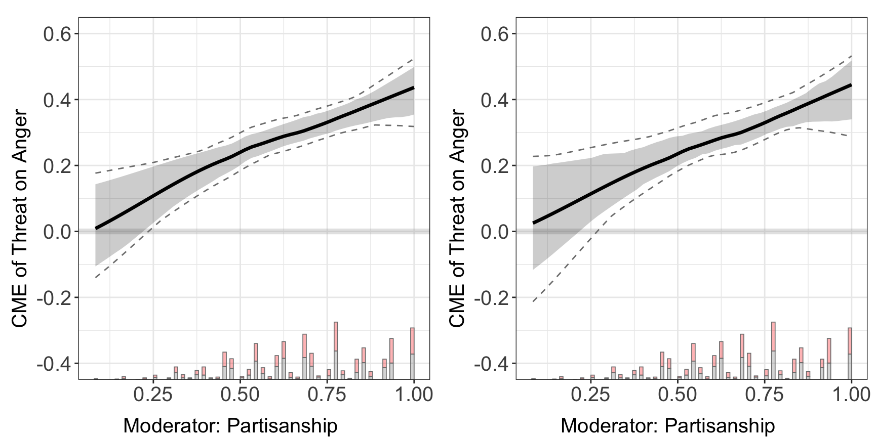
4.1.0.2.3 Smoothing options
To transform the signal—which is one value per unit—into a smooth one‐dimensional CME along the moderator \(X\), the AIPW‐Lasso estimator uses dimension reduction. You can either fit a linear model of the signal on a B‐spline basis of \(X\) via reduce.dimension = bspline, or fit a local‐kernel smoother of the signal on \(X\) via reduce.dimension = kernel (default).
aipw.out.bs.smooth <- interflex(estimator = "lasso", data = d,
                 Y = Y,D = D, X = X, Z = Z,
                 Ylabel = Ylabel, Dlabel = Dlabel,
                 Xlabel = Xlabel,
                 reduce.dimension = "bspline",
                 main = "Smoothing: b-spline")
#> Parallel computing: using 8 of 14 available cores.
#> To change: set cores = <n> in interflex().
#> Baseline group not specified; choose treat = 0 as the baseline group.
#> >> Treatment is binary/discrete.
#>    Signal = aipw
#>    Estimand = ATE
#>    Basis extension = bspline
#>    Outcome model = lasso; PS model = lasso
#> Step 1: Matching arguments and setting defaults...
#> Step 2: Performing basic checks on input data...
#> Step 3: Processing fixed effects (if provided)...
#> Step 4: Setting up evaluation grid for X (if not provided)...
#> Step 5: Building design matrix...
#> Design matrix successfully built.
#> Step 6: Setting up model types based on signal argument...
#> Step 7: Fitting outcome and propensity score models...
#>    Fitting outcome model for treated (D=1) units...
#>    Fitting propensity score model (no FE)...
#> Step 8: Performing post-lasso variable selection (if applicable)...
#>    Post-lasso: refitting outcome and propensity score models on selected variables...
#> Step 9: Generating predictions from fitted models...
#> Step 10: Computing signals and performing dimension reduction...
#> Step 11: Estimation complete. Returning results.

aipw.out.bs.kernel <- interflex(estimator = "lasso", data = d,
                  Y = Y,D = D, X = X, Z = Z,
                  Ylabel = Ylabel, Dlabel = Dlabel,
                  Xlabel = Xlabel,
                  reduce.dimension = "kernel",
                  main = "Smoothing: kernel")
#> Parallel computing: using 8 of 14 available cores.
#> To change: set cores = <n> in interflex().
#> Baseline group not specified; choose treat = 0 as the baseline group.
#> >> Treatment is binary/discrete.
#>    Signal = aipw
#>    Estimand = ATE
#>    Basis extension = bspline
#>    Outcome model = lasso; PS model = lasso
#> Step 1: Matching arguments and setting defaults...
#> Step 2: Performing basic checks on input data...
#> Step 3: Processing fixed effects (if provided)...
#> Step 4: Setting up evaluation grid for X (if not provided)...
#> Step 5: Building design matrix...
#> Design matrix successfully built.
#> Step 6: Setting up model types based on signal argument...
#> Step 7: Fitting outcome and propensity score models...
#>    Fitting outcome model for treated (D=1) units...
#>    Fitting propensity score model (no FE)...
#> Step 8: Performing post-lasso variable selection (if applicable)...
#>    Post-lasso: refitting outcome and propensity score models on selected variables...
#> Step 9: Generating predictions from fitted models...
#> Step 10: Computing signals and performing dimension reduction...
#> Step 11: Estimation complete. Returning results.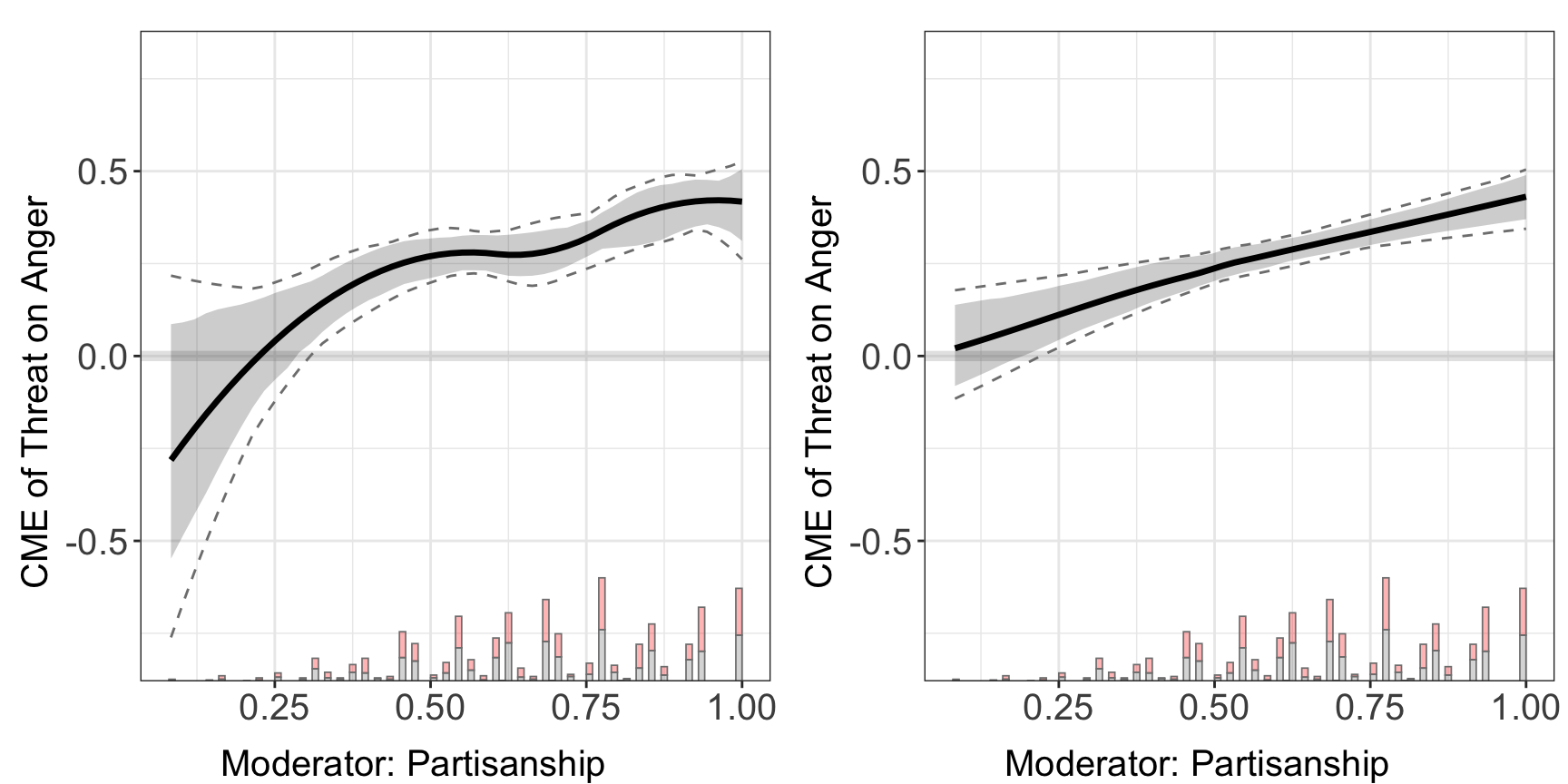
4.1.0.2.4 Basis expansions options
In fitting the outcome and propensity score models, we introduce basis expansions to relax parametric assumptions and enhance estimation flexibility. The basis expansion provides several options via basis.type, expanding the set of regressors \(V = (X, Z)\) beyond their raw forms. When basis.type = "none", \(V = (X, Z)\) enters the design matrix in its raw form; when basis.type = "polynomial", every numeric entry in \(V=(X,Z)\) is expanded to its first two global powers; and when basis.type = "bspline" (default), each variable is replaced with piecewise polynomials that bend only near their knots. The option include.interactions = TRUE (default) adds interaction terms among these expanded basis functions as additional covariates.
aipw.out.poly.basis <- interflex(estimator = "lasso", data = d,
                        Y = Y,D = D, X = X, Z = Z,
                        Ylabel = Ylabel, Dlabel = Dlabel, Xlabel = Xlabel,
                        basis.type = 'polynomial')
#> Parallel computing: using 8 of 14 available cores.
#> To change: set cores = <n> in interflex().
#> Baseline group not specified; choose treat = 0 as the baseline group.
#> >> Treatment is binary/discrete.
#>    Signal = aipw
#>    Estimand = ATE
#>    Basis extension = polynomial
#>    Outcome model = lasso; PS model = lasso
#> Step 1: Matching arguments and setting defaults...
#> Step 2: Performing basic checks on input data...
#> Step 3: Processing fixed effects (if provided)...
#> Step 4: Setting up evaluation grid for X (if not provided)...
#> Step 5: Building design matrix...
#> Design matrix successfully built.
#> Step 6: Setting up model types based on signal argument...
#> Step 7: Fitting outcome and propensity score models...
#>    Fitting outcome model for treated (D=1) units...
#>    Fitting propensity score model (no FE)...
#> Step 8: Performing post-lasso variable selection (if applicable)...
#>    Post-lasso: refitting outcome and propensity score models on selected variables...
#> Step 9: Generating predictions from fitted models...
#> Step 10: Computing signals and performing dimension reduction...
#> Step 11: Estimation complete. Returning results.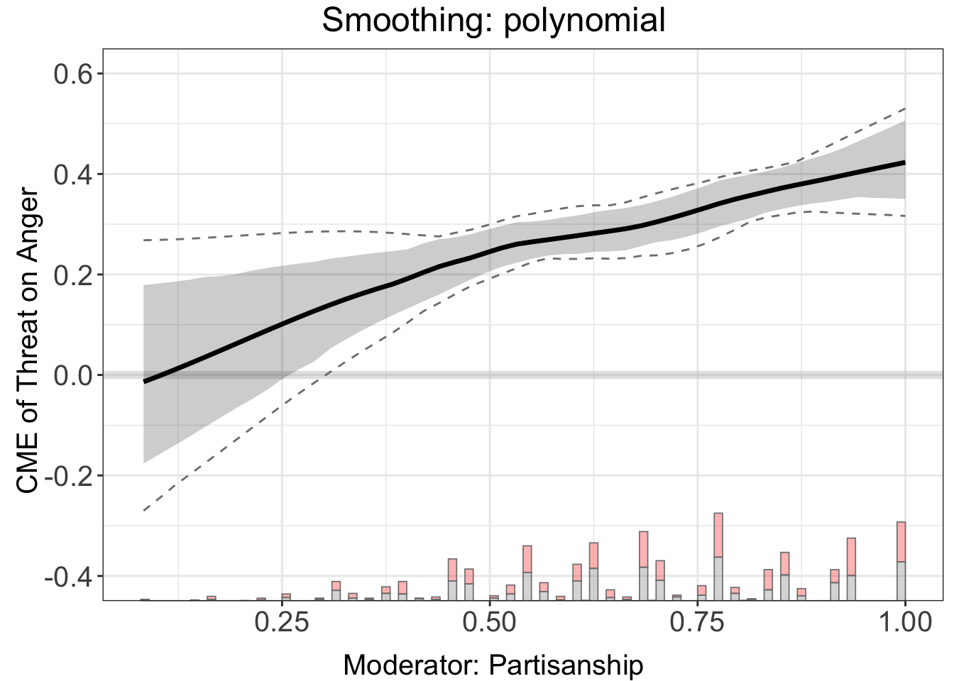
4.2 Continuous treatment
With continuous treatment, we use the empirical example from Adiguzel et al. (2023). The outcome is the change in vote share for the incumbent AKP party; the treatment is the change in congestion, measured by the number of patients per doctor at the nearest clinic; and the moderator is the logarithm of median property value.
In settings with continuous treatment, there is no propensity score model to estimate. Instead, we adopt a partially linear regression model (PLRM), where we regress \(\tilde{Y}\) on \(\tilde{D}\) after “partialling out” the effect of covariates \(V\) from outcome \(Y\) and treatment \(D\).
In practice, we estimate the relationships between outcome \(Y\) and covariates \(V = (X, Z)\) and between treatment \(D\) and covariates \(V\) separately, using flexible models such as basis expansions combined with post‐selection Lasso to denoise \(Y\) and \(D\) into \(\tilde{Y}\) and \(\tilde{D}\). Hence, the estimator is named the Partial‐Out Lasso estimator.
data(app_adiguzel2023)
#> Warning in data(app_adiguzel2023): data set 'app_adiguzel2023' not found
d<-app_adiguzel2023
d<-remove_labels(d)
d<-as.data.frame(d)
main<-"Adiguzel2023a"
D="Dwalk_3"
Y="Dakp_3"
X="lograyic09"

Z=c('Duniversity_3', 'Dodr_3', 'Dydr_3', 'Dpopulation_3', 'Dhospital_pri_3', 'Dhospital_pub_3')

Dlabel<-"Dwalk"
Ylabel<-"Dakp"
Xlabel<-"Property values (2009)"
4.2.0.1 PO-Lasso estimator
Estimation. The syntax to deploy the PO‐Lasso estimator is the same as in the binary‐treatment setting: specify estimator = "lasso". Both pointwise and uniform CIs are provided in the plot.
Results. Similarly, estimation results and the plot can be extracted from the output object.
aipw.out.1 <- interflex(estimator = "lasso", data = d,
                 Y = Y,D = D, X = X, Z = Z,
                 Ylabel = Ylabel, Dlabel = Dlabel,
                 Xlabel = Xlabel,
                 main = "AIPW estimation")
#> Parallel computing: using 8 of 14 available cores.
#> To change: set cores = <n> in interflex().
#> >> Treatment is continuous.
#>    Outcome model = lasso; Treatment model = lasso
#>    Basis extension = bspline
#> BootstrapPLR Step 1: Fitting full-sample PLR model...
#> Step 0: Checking inputs and extracting variables...
#> Step 1: Building or validating design matrix (including FE)...
#>   -> Design matrix built with 400 columns (including FE dummies).
#> Step 2: Identifying FE columns and building penalty factors...
#>   -> No FE specified; penalty factors default to NULL (full penalty).
#> Step 3: Fitting outcome and treatment models...
#>   -> Fitting outcome model (type = lasso )...
#>   -> Fitting treatment model (type = lasso )...
#> Step 4: Performing post-selection if LASSO/Ridge was used...
#> Step 5: Generating predictions and residual signals...
#> Step 6: Estimating CME curve via kernel ...
#>   -> Running kernel-based conditional ATE via interflex::interflex()
#> Cross-validating bandwidth ...
#> Optimal bw=7.8836.
#> Number of evaluation points:50
#>   -> Selected bandwidth = 7.883621
#>   -> CME estimation on grid complete.
#> Step 7: Returning results.
#>   -> Full-sample fit complete.
#>   -> Using bandwidth = 7.883621
#> BootstrapPLR Step 2: Preparing for 200 bootstrap draws...
#> BootstrapPLR Step 3: Setting up parallel backend...
#> BootstrapPLR Step 4: Running bootstrap loop...
#>   -> Bootstrap loop complete.
#> BootstrapPLR Step 5: Computing pointwise SEs and CIs...
#> BootstrapPLR Step 6: Computing uniform CIs...
#> BootstrapPLR Step 7: Assembling output...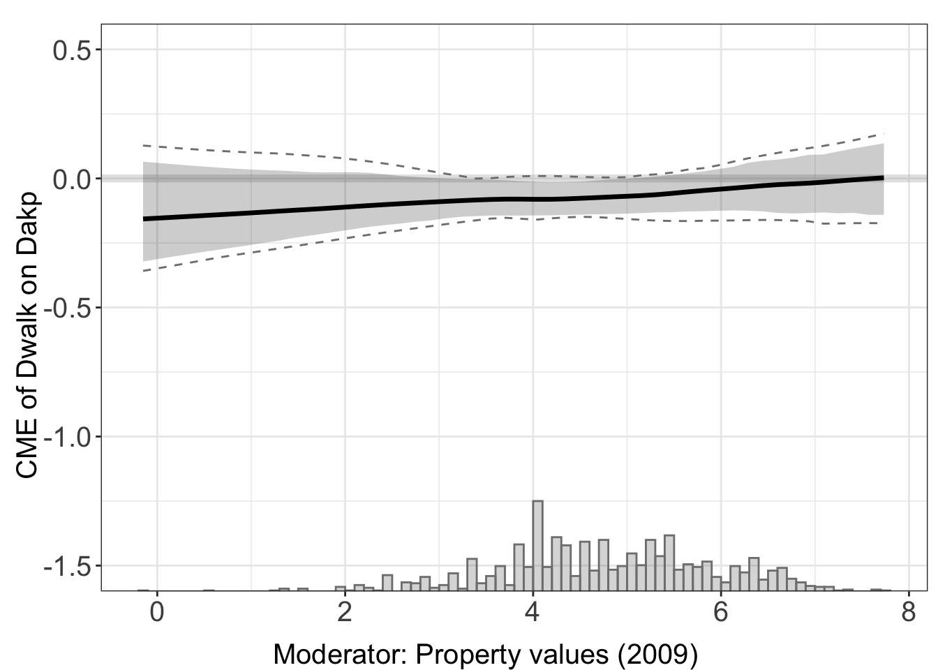
head(aipw.out.1$est.lasso[[1]])
#>             X        CME         SE   CI.lower   CI.upper CI.lower.uniform
#> 1 -0.15082289 -0.1569029 0.09767628 -0.3217683 0.06496761       -0.3582830
#> 2  0.01006734 -0.1536706 0.09450500 -0.3120129 0.06025213       -0.3480930
#> 3  0.17095758 -0.1504513 0.09128132 -0.3024535 0.05512992       -0.3378921
#> 4  0.33184781 -0.1471550 0.08815027 -0.2934947 0.05040896       -0.3273443
#> 5  0.49273804 -0.1438398 0.08511095 -0.2846195 0.04613766       -0.3167496
#> 6  0.65362828 -0.1405853 0.08211801 -0.2759353 0.04208881       -0.3064470
#>   CI.upper.uniform
#> 1        0.1274071
#> 2        0.1231508
#> 3        0.1186429
#> 4        0.1143653
#> 5        0.1105306
#> 6        0.1069637
4.2.1 Advanced options
With continuous treatment, we also provide a set of advanced options tailored to the user’s research needs. These include:
basis.type: As in the binary‐treatment case, you can choose among none, polynomial, or bspline to control how \(V=(X,Z)\) is expanded in the first‐stage regressions.
include.interactions: When set to TRUE (the default), interaction terms among all basis‐expanded covariates are included.
reduce.dimension: After partialling out, you can smooth the signal via B‐splines (bspline) or a local‐kernel smoother (kernel).
The estimand and signal options are not supported.
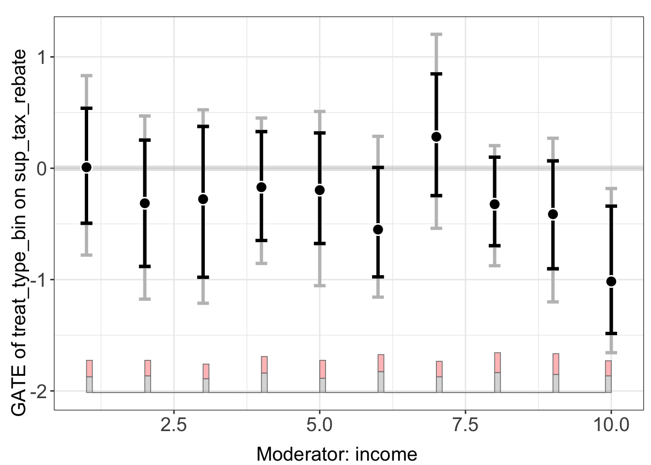
4.3 GATE with discrete moderator
When the moderator \(X\) is discrete, we can estimate Group Average Treatment Effects (GATE) by setting gate = TRUE. This computes the average treatment effect within each level of \(X\) using the AIPW-Lasso framework.
We use the Beiser-McGrath and Bernauer (2024) example with income as a discrete moderator:
data(app_bb2024)
d <- app_bb2024
d <- remove_labels(d)

out.lasso.gate <- interflex(estimator = 'lasso', data = d,
                            Y = "sup_tax_rebate", D = "treat_type_bin",
                            X = "income", Z = c("leftright", "clim_belief", "resp_age", "female", "employment_f", "highedu", "midedu", "pid_f"),
                            na.rm = TRUE, gate = TRUE)
#> Parallel computing: using 8 of 14 available cores.
#> To change: set cores = <n> in interflex().
#> Baseline group not specified; choose treat = 0 as the baseline group.
#> >> Treatment is discrete/binary.
#>    Signal     = aipw
#>    Estimand   = ATE
#>    Basis type = none
#>    Outcome model   = lasso ; Propensity model = lasso
#> Design matrix built
#> Fitting outcome models...
#> Fitting propensity model...out.lasso.gate$figure
Use plot(..., by.group = TRUE) for a clearer visualization with separate point estimates and confidence intervals per group:
plot(out.lasso.gate, by.group = TRUE)