d<-app_hma2015

Y = "totangry" ## outcome: anger
D = "threat" ## treatment: threat
X = "pidentity" ## moderator: partisan identity
Z <-  c("issuestr2", "knowledge", "educ","male", "age10")

Ylabel = "Anger"
Dlabel = "Threat"
Xlabel = "Partisanship"5 Double Machine Learning
This chapter gives a brief overview of estimating CMEs using the interflex pacakge, focusing on the Double/debiased Machine Learning (DML) estimator. This chapter walks through using DML estimators for different empirical setup with real-world data, including binary treatment and continuous treatment.
5.1 Overview
When treatment \(D\), moderator \(X\) and covariates\(Z\) are all discrete, we can estimate the CME nonparametrically. However, when one of them is continuous or high-dimensional, CME becomes difficult to estimate without imposing functional form assumptions. These assumptions can be too restrictive and easily violated in practice.
Here, we introduce the double/debiased machine learning (DML) estimator, to flexibly estimate CME under mild conditions. The primary advantage of DML lies in its ability to use machine learning method to estimate nuisance parameters \(\eta_0\) (parameters that are not of direct interest to researchers), in nonparametric, data-driven way, while providing valid inference for the target quantity, in this case, the CME \(\theta_0\).
The DML framework operates through the following steps:
1. Estimate nuisance functions
- Outcome model: Estimate the nuisance function that captures relationship between outcome \(Y\) covariate \(V = (X, Z)\), using ML methods.
- Treatment model: Estimate the nuisance function that captures relationship between treatment \(D\) covariate \(V = (X, Z)\).
2. Construct signals The key of DML estimator is the construction of orthogonal score to meet the Neyman orthogonality condition. With binary treatment, the signal is constructed through AIPW correction; With continuous treatment, the signal is constructed via “partialling out”.
3. Dimension reduction
The constructed orthogonal signal is projected onto a functional space in \(X\), which, in the interflex package, is either a B-spline or kernel regression, to recover CME.
When setting the option estimator to dml, the function will conduct the two-stage DML estimator to compute the marginal effects. In the following command, the outcome variable is \(Y\), the moderator is \(X\), the covariates are \(Z\).
5.2 Binary treatment
In the binary treatment setting, we are using the Huddy et al. (2015) example, with outcome variable being level of anger, treatment variable being electoral loss threat or electoral win reassurance, and moderator \(X\) is strength of partisan identity.
Estimation. To implement the DML estimator, we need to set the option estimator="dml" and specify two machine learning models: one for the outcome model (via the option model.y) and one for the treatment model (via the option model.t). treat.type set the data type of treatment variable, it can be either continuous or discrete, the default is discrete.
Here, we use a neural network model (nn) for the outcome model and a random forest model (rf) for the treatment model. The gray area depicts the pointwise interval, while the dashed line marks the uniform/joint confidence interval.
binary.dml.nn.rf <- interflex(estimator="dml", data = d,
                              Y = Y, D = D, X = X, Z = Z,
                              Ylabel = Ylabel, Dlabel = Dlabel, Xlabel = Xlabel,
                              model.y = "nn",model.t = "rf")
#> Parallel computing: using 8 of 14 available cores.
#> To change: set cores = <n> in interflex().
#> Baseline group not specified; choose treat = 0 as the baseline group.plot(binary.dml.nn.rf)
#> Warning: Using `size` aesthetic for lines was deprecated in ggplot2 3.4.0.
#> ℹ Please use `linewidth` instead.
#> ℹ The deprecated feature was likely used in the interflex package.
#> Please report the issue to the authors.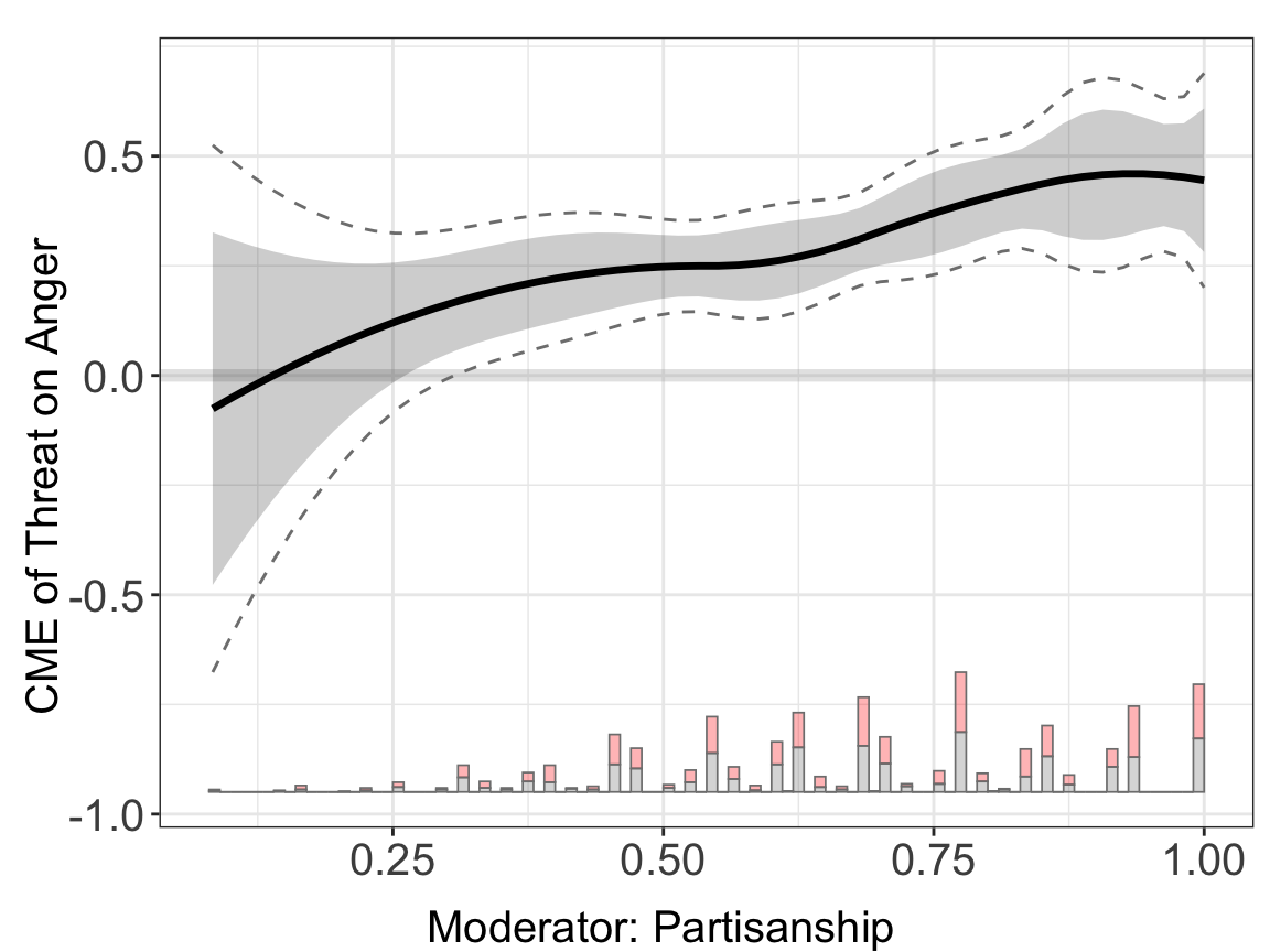
Results. The estimated treatment effects of \(D\) on \(Y\) across the support of \(X\) are saved in:
## printing the first 10 rows
lapply(binary.dml.nn.rf$est.dml, head, 10)
#> $`1`
#>             X            ME         sd lower CI(95%) upper CI(95%)
#> 1  0.08333334 -7.585085e-02 0.20509878   -0.47783707     0.3261354
#> 2  0.10204082 -4.941964e-02 0.18311691   -0.40832218     0.3094829
#> 3  0.12074830 -2.410749e-02 0.16271719   -0.34302733     0.2948124
#> 4  0.13945578  8.559899e-05 0.14394597   -0.28204331     0.2822145
#> 5  0.15816327  2.315963e-02 0.12686024   -0.22548187     0.2718011
#> 6  0.17687075  4.511459e-02 0.11152821   -0.17347668     0.2637059
#> 7  0.19557823  6.595049e-02 0.09802703   -0.12617895     0.2580799
#> 8  0.21428572  8.566734e-02 0.08643469   -0.08374154     0.2550762
#> 9  0.23299320  1.042651e-01 0.07681176   -0.04628316     0.2548134
#> 10 0.25170068  1.217438e-01 0.06916990   -0.01382668     0.2573144
#>    lower uniform CI(95%) upper uniform CI(95%)
#> 1            -0.67637727             0.5246756
#> 2            -0.58558343             0.4867442
#> 3            -0.50054120             0.4523262
#> 4            -0.42138622             0.4215574
#> 5            -0.34828541             0.3946047
#> 6            -0.28143847             0.3716677
#> 7            -0.22107130             0.3529723
#> 8            -0.16741225             0.3387469
#> 9            -0.12063865             0.3291689
#> 10           -0.08078469             0.3242724
5.2.1 First Stage DML Model Selections
The dml estimator supports five different machine learning algorithms: linear (Linear model), regularization (Lasso or Ridge model),rf (Random Forest), nn (Neural Network), and hgb (Histogram-based Gradient Boosting). Users can change the model.y and model.t option to calculate the nuisance parameter using a different ML method.
## linear + linear
binary.dml.ln.ln <- interflex(estimator="dml", data = d,
                              Y = Y, D = D, X = X, Z = Z,
                              Ylabel = Ylabel, Dlabel = Dlabel,
                              Xlabel = Xlabel,
                              model.y = "linear",model.t = "linear",
                              main = "Linear Model")
#> Parallel computing: using 8 of 14 available cores.
#> To change: set cores = <n> in interflex().
#> Baseline group not specified; choose treat = 0 as the baseline group.

## neural network + neural network
binary.dml.nn.nn <- interflex(estimator="dml", data = d,
                              Y = Y, D = D, X = X, Z = Z,
                              Ylabel = Ylabel, Dlabel = Dlabel,
                              Xlabel = Xlabel,
                              model.y = "nn",model.t = "nn",
                              main = "Neural Network: Default")
#> Parallel computing: using 8 of 14 available cores.
#> To change: set cores = <n> in interflex().
#> Baseline group not specified; choose treat = 0 as the baseline group.


## random forest + random forest
binary.dml.rf.rf <- interflex(estimator="dml", data = d,
                              Y = Y, D = D, X = X, Z = Z,
                              Ylabel = Ylabel, Dlabel = Dlabel,
                              Xlabel = Xlabel,
                              model.y = "rf",model.t = "rf",
                              main = "Random Forest")
#> Parallel computing: using 8 of 14 available cores.
#> To change: set cores = <n> in interflex().
#> Baseline group not specified; choose treat = 0 as the baseline group.

## hist gradient boosting + hist gradient boosting
binary.dml.hgb.hgb <- interflex(estimator="dml",data = d,
                              Y = Y, D = D, X = X, Z = Z,
                              Ylabel = Ylabel, Dlabel = Dlabel,
                              Xlabel = Xlabel,
                              model.y = "hgb",model.t = "hgb",
                              main = "Hist Gradient Boosting")
#> Parallel computing: using 8 of 14 available cores.
#> To change: set cores = <n> in interflex().
#> Baseline group not specified; choose treat = 0 as the baseline group.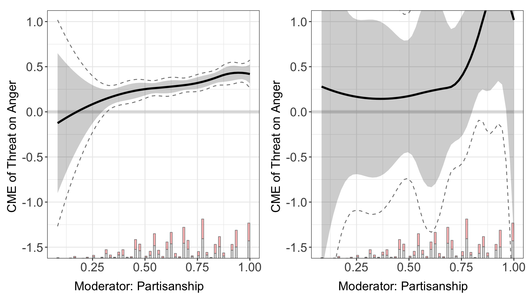
#>
#> $`2`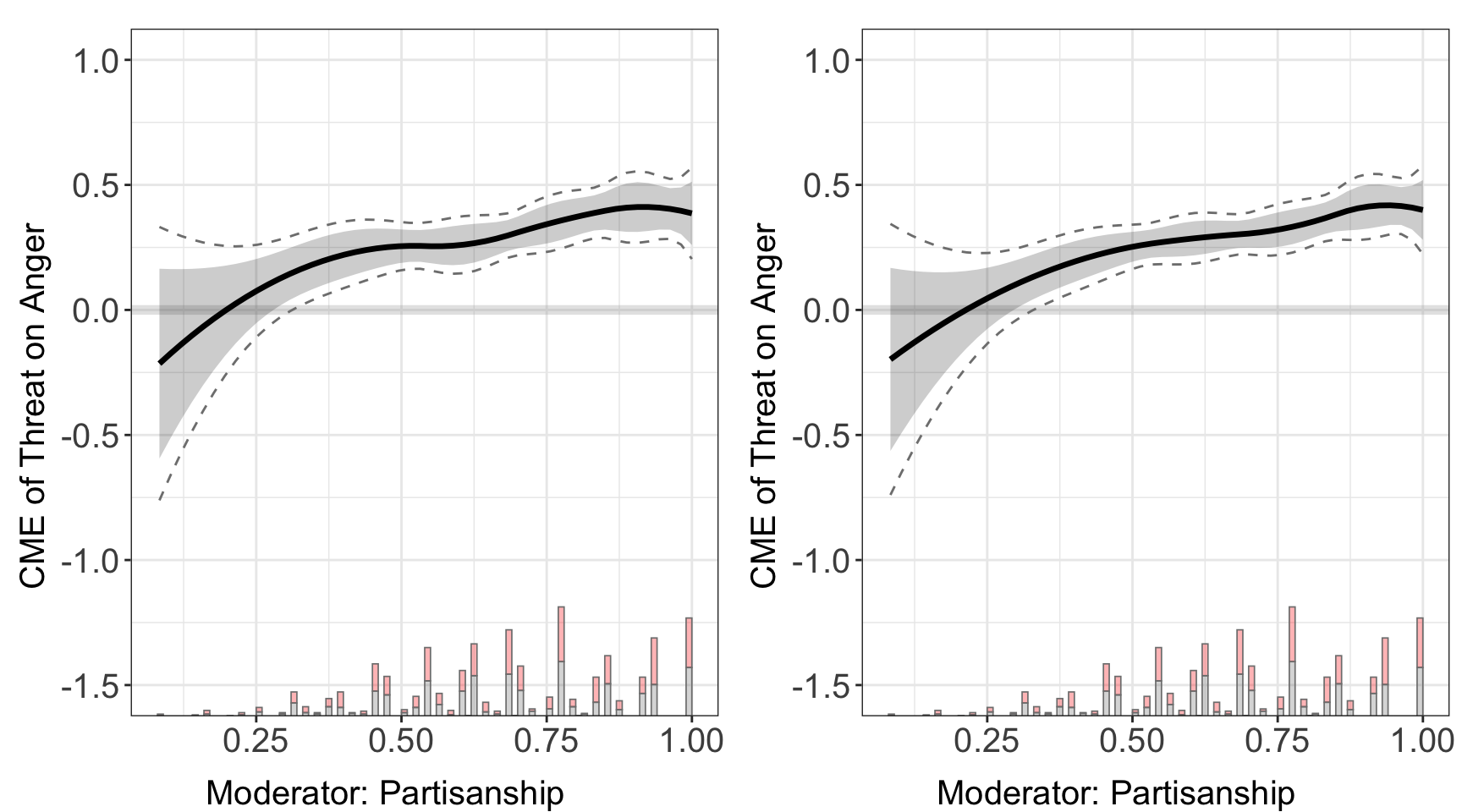
#>
#> attr(,"class")
#> [1] "list"      "ggarrange"
We find that different ML models give very similar results, which is expected since all methods can accurately partial out their impacts on the outcome and the treatment.
5.2.2 Model Parameters
Users can customize parameters for the machine learning model in both stages by specifying the options param.y and param.t. For the linear method, users can refer to the LinearRgression and LogisticRegression if outcome is discrete. For the lasso method, please refere to LogisticRegression with default regularization. For the whole list of parameters that are applicable to the neural network model, users can refer to the MLPRegressor or the MLPClassifier. For the random forest method, users can refer to the RandomForestRegressor or the RandomForestClassifier. For the hist gradient boosting method, users can refer to the HistGradientBoostingRegressor or the HistGradientBoostingClassifier.
Here we use Huddy (2015) to explore how selecting different DML parameters affects performance. We can directly specify the size of the neural networks, the activation function, learning rate, and solver using the list param_nn and feed them to the DML estimator. We compare it with the DML estimator using nn as first stage model, but without adjusting parameters.
param_nn <- list(
  hidden_layer_sizes = list(10L,20L,10L),
  activation = c("tanh"),
  solver = c("sgd"),
  alpha = c(0.05),
  learning_rate = c("adaptive")
)

binary.dml.nn.linear.para <- interflex(estimator="dml", data = d,
                              Y = Y, D = D, X = X, Z = Z,
                              Ylabel = Ylabel, Dlabel = Dlabel,
                              Xlabel = Xlabel,
                              model.y = "nn", param.y = param_nn,
                              model.t = "nn", param.t = param_nn,
                              main = "Neural Network: Fine-tuned")
#> Parallel computing: using 8 of 14 available cores.
#> To change: set cores = <n> in interflex().
#> Baseline group not specified; choose treat = 0 as the baseline group.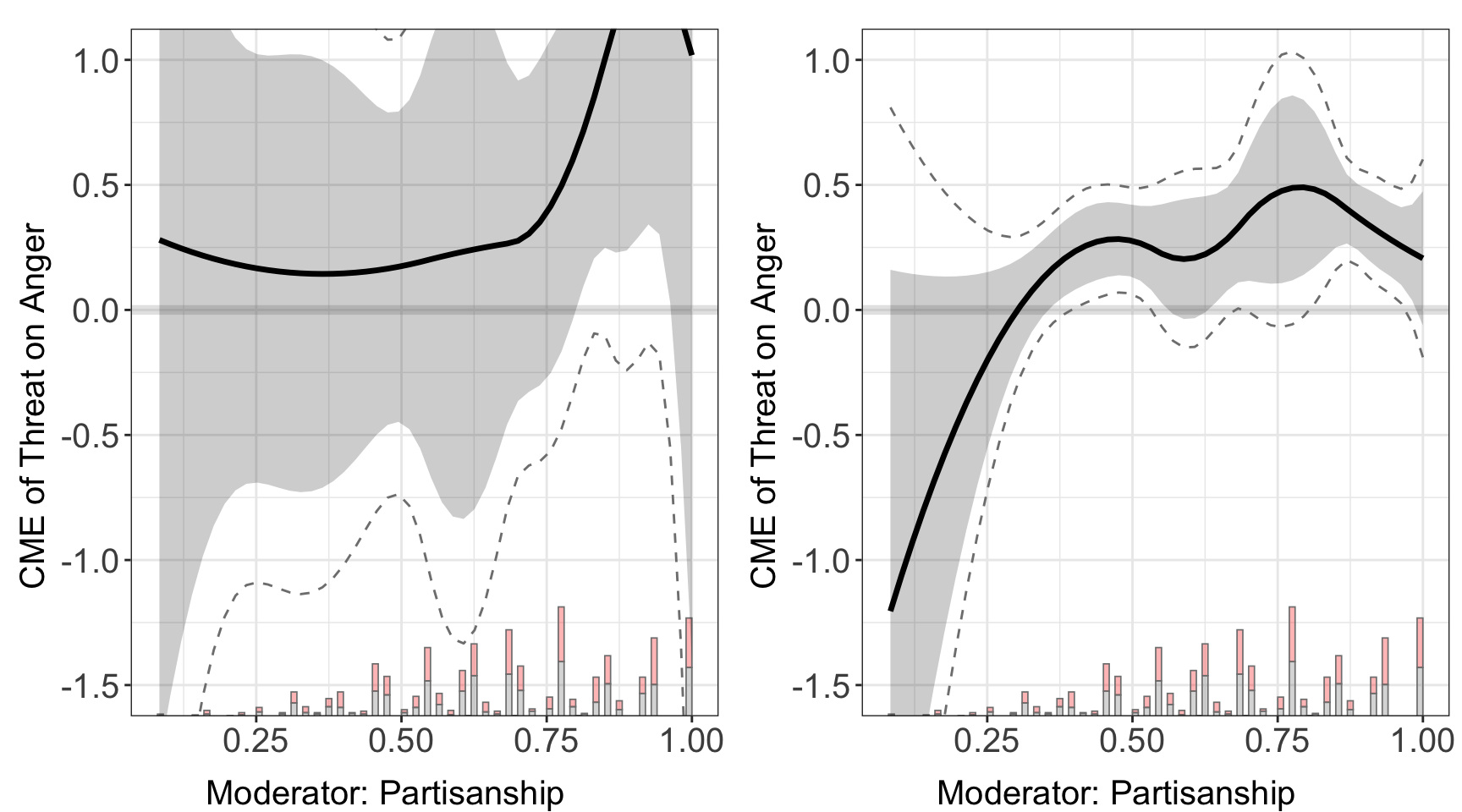
5.2.3 Cross-Validation
Users can also specify the grids of parameters using the options param.grid.y and param.grid.t. The DML estimator will then search through all sequences of parameter settings and pick the most suitable one using cross-validation. We need to set the options CV to TRUE to invoke the cross-validation. As an example, we specify the grids used for the lasso/ridge regression, neural network, random forest, and hist gradient boosting, then we compare their performances on Huddy et al. (2015).
param_grid_nn <- list(
  hidden_layer_sizes = list(list(10L,20L,10L), list(20L)),
  activation = c("tanh","relu"),
  solver = c("sgd","adam"),
  alpha = c(0.0001,0.05),
  learning_rate = c("constant","adaptive")
)

param_grid_rf <- list(
  max_depth = c(2L,3L,5L,7L),
  n_estimators = c(10L, 30L, 50L, 100L, 200L, 400L, 600L, 800L, 1000L),
  max_features = c(1L,2L)
)

param_grid_hgb <- list(
  max_leaf_nodes = c(5L,10L,20L,30L),
  min_samples_leaf = c(5L,10L,20L),
  l2_regularization = c(0,0.1,0.5),
  max_features = c(0.5,1)
)


# nn (cv) + rf (cv) + linear
binary.cvnn.cvrf <- interflex(estimator="dml", data = d,
                              Y = Y, D = D, X = X, Z = Z,
                              Ylabel = Ylabel, Dlabel = Dlabel,
                              Xlabel = Xlabel,CV = TRUE,
                              model.y = "nn",param.grid.y = param_grid_nn,
                              model.t = "rf",param.grid.t = param_grid_rf)
#> Parallel computing: using 8 of 14 available cores.
#> To change: set cores = <n> in interflex().
#> Baseline group not specified; choose treat = 0 as the baseline group.

# nn (cv) + hgb (cv) + regularization (cv)
binary.cvnn.cvhgb <- interflex(estimator="dml", data = d,
                              Y = Y, D = D, X = X, Z = Z,
                              Ylabel = Ylabel, Dlabel = Dlabel,
                              Xlabel = Xlabel,CV = TRUE,
                              model.y = "nn",param.grid.y = param_grid_nn,
                              model.t = "hgb",param.grid.t = param_grid_hgb)
#> Parallel computing: using 8 of 14 available cores.
#> To change: set cores = <n> in interflex().
#> Baseline group not specified; choose treat = 0 as the baseline group.

# rf (cv) + rf (cv) + rf (cv)
binary.cvrf.cvrf <- interflex(estimator="dml", data = d,
                              Y = Y, D = D, X = X, Z = Z,
                              Ylabel = Ylabel, Dlabel = Dlabel,
                              Xlabel = Xlabel,CV = TRUE,
                              model.y = "rf",param.grid.y = param_grid_rf,
                              model.t = "rf",param.grid.t = param_grid_rf)
#> Parallel computing: using 8 of 14 available cores.
#> To change: set cores = <n> in interflex().
#> Baseline group not specified; choose treat = 0 as the baseline group.

# hgb (cv) + hgb (cv) + hgb (cv)
binary.cvhgb.cvhgb <- interflex(estimator="dml",  data = d,
                              Y = Y, D = D, X = X, Z = Z,
                              Ylabel = Ylabel, Dlabel = Dlabel,
                              Xlabel = Xlabel,CV = TRUE,
                              model.y = "hgb",param.grid.y = param_grid_hgb,
                              model.t = "hgb",param.grid.t = param_grid_hgb)
#> Parallel computing: using 8 of 14 available cores.
#> To change: set cores = <n> in interflex().
#> Baseline group not specified; choose treat = 0 as the baseline group.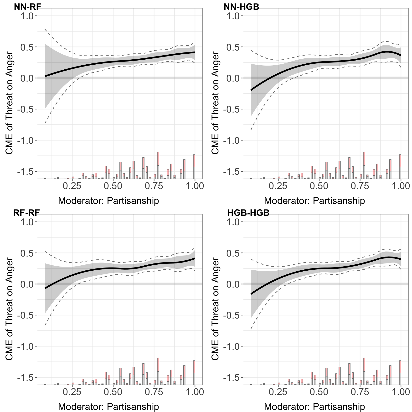
5.2.4 Comparison of estimators
In this section, we compare the performance of DML estimator with previously introduced estimators.
out.linear<-interflex(estimator = "binning",Y=Y,D=D,
                    X=X,Z=Z,data=d, Xlabel=Xlabel,
                    Ylabel=Ylabel, Dlabel=Dlabel,
                    ylim = c(-1.5, 1))
#> Baseline group not specified; choose treat = 0 as the baseline group.

out.kernel<-interflex(estimator = "kernel", data=d, Y=Y,D=D,X=X,Z=Z,
                      vartype = 'bootstrap', parallel = TRUE,
                      Dlabel=Dlabel, Xlabel=Xlabel, Ylabel=Ylabel,
                      ylim = c(-1.5, 1))
#> Parallel computing: using 8 of 14 available cores.
#> To change: set cores = <n> in interflex().
#> Baseline group not specified; choose treat = 0 as the baseline group.
#> Cross-validating bandwidth ...
#> Optimal bw=0.9167.
#> Number of evaluation points:50

out.aipw <- interflex(estimator = "lasso", Y=Y,D=D,X=X,data=d,
                     Xlabel=Xlabel, Ylabel=Ylabel, Dlabel=Dlabel,
                     ylim = c(-1.5, 1))
#> Parallel computing: using 8 of 14 available cores.
#> To change: set cores = <n> in interflex().
#> Baseline group not specified; choose treat = 0 as the baseline group.
#> >> Treatment is binary/discrete.
#>    Signal = aipw
#>    Estimand = ATE
#>    Basis extension = bspline
#>    Outcome model = lasso; PS model = lasso
#> Step 1: Matching arguments and setting defaults...
#> Step 2: Performing basic checks on input data...
#> Step 3: Processing fixed effects (if provided)...
#> Step 4: Setting up evaluation grid for X (if not provided)...
#> Step 5: Building design matrix...
#> Design matrix successfully built.
#> Step 6: Setting up model types based on signal argument...
#> Step 7: Fitting outcome and propensity score models...
#>    Fitting outcome model for treated (D=1) units...
#>    Fitting propensity score model (no FE)...
#> Step 8: Performing post-lasso variable selection (if applicable)...
#>    Post-lasso: refitting outcome and propensity score models on selected variables...
#> Step 9: Generating predictions from fitted models...
#> Step 10: Computing signals and performing dimension reduction...
#> Step 11: Estimation complete. Returning results.ggarrange(out.linear$figure, out.kernel$figure,
out.aipw$figure, binary.cvnn.cvrf$figure,
common.legend = TRUE, legend = "none",
labels = c("Binning", "Kernel", "AIPW-Lasso", "DML: NN-RF"))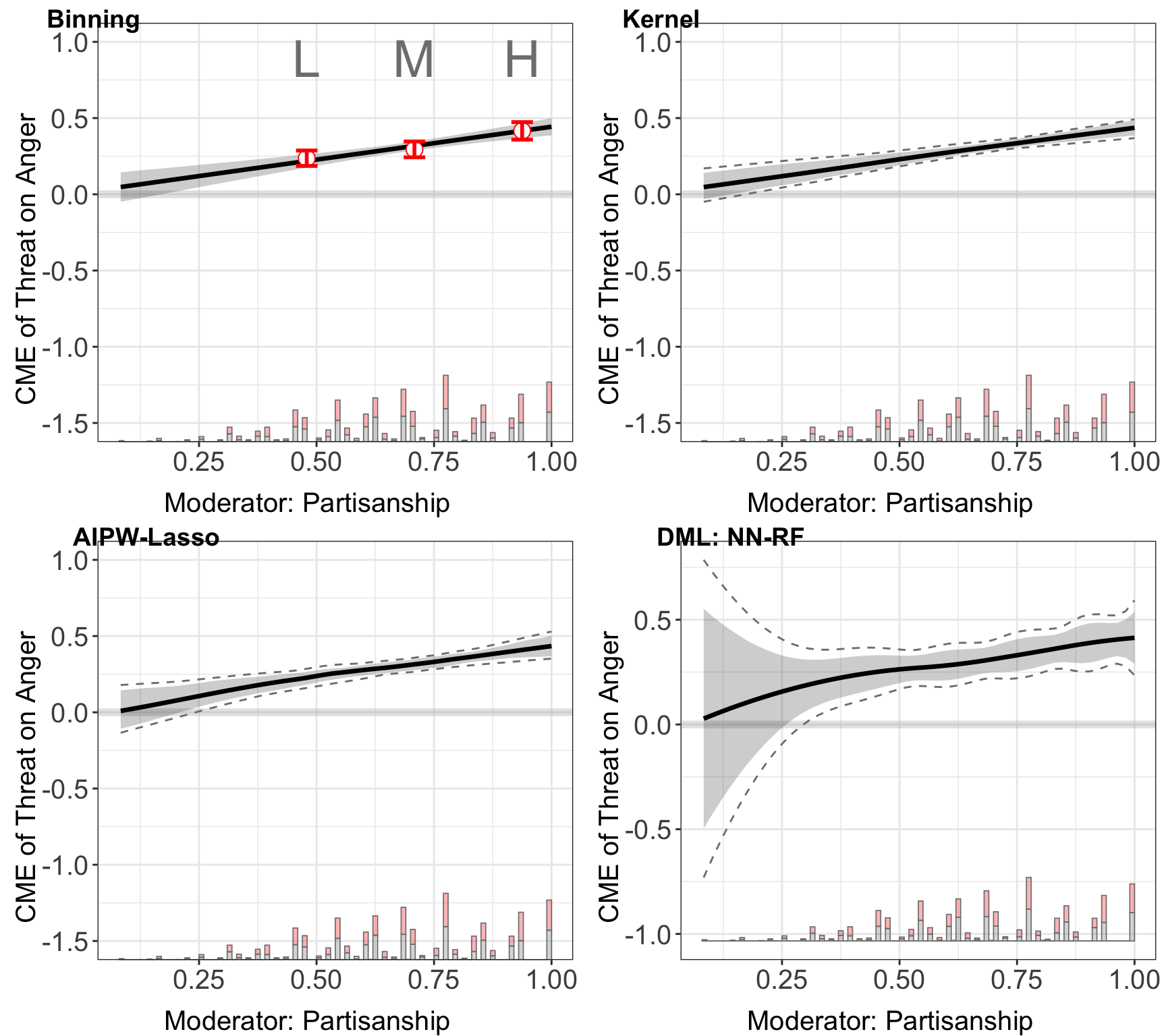
These plots consistently show that the CME of the threat on anger escalates with increasing partisan identity across all machine learning methods employed.
5.3 Continuous Treatment
In this section, we demonstrate the application of the DML estimator, focusing on scenarios with continuous treatment. We use the previous empirical example from Adiguzel et al. (2023). The outcome is change in the vote share for the incumbent AKP party, treatment is change in congestion, measured by the number of patients per doctor at the nearest clinic, moderator is logarithm of median property value.
data(app_adiguzel2023)
#> Warning in data(app_adiguzel2023): data set 'app_adiguzel2023' not found
d<-app_adiguzel2023
d<-remove_labels(d)
d<-as.data.frame(d)
main<-"Adiguzel2023a"
D="Dwalk_3"
Y="Dakp_3"
X="lograyic09"

Z=c('Duniversity_3', 'Dodr_3', 'Dydr_3', 'Dpopulation_3', 'Dhospital_pri_3', 'Dhospital_pub_3')

Dlabel<-"Dwalk"
Ylabel<-"Dakp"
Xlabel<-"Property values (2009)"
With continuous treatment, we need to specify the data type in treat.type = continuous. The estimator automatically plots both the pointwise and uniform CI.
cont.dml<- interflex(estimator="dml", data = d,
                    Y = Y, D = D, X = X, Z = Z,
                    Ylabel = Ylabel, Dlabel = Dlabel,
                    Xlabel = Xlabel,
                    treat.type = "continuous")
#> Parallel computing: using 8 of 14 available cores.
#> To change: set cores = <n> in interflex().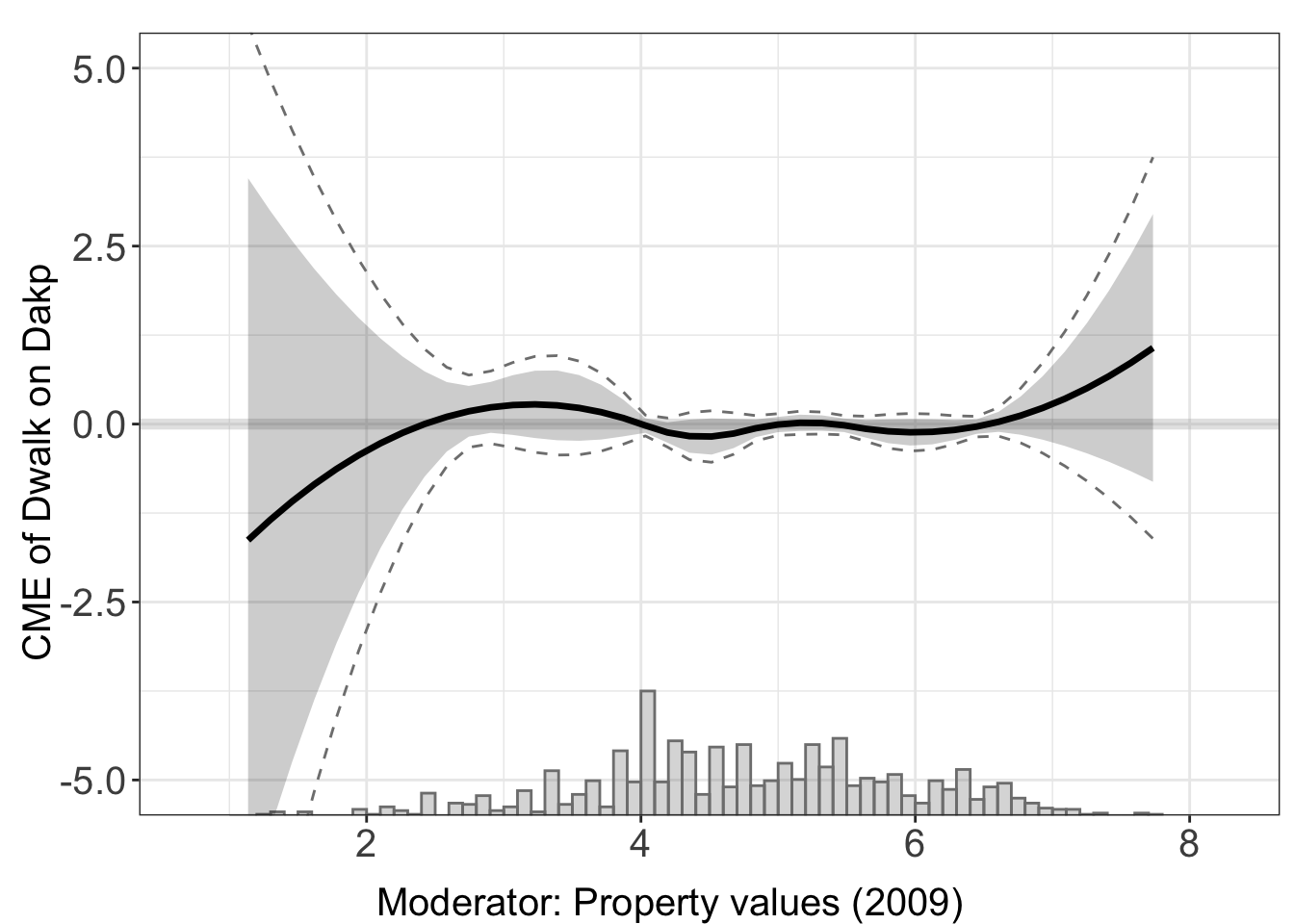
We can access the results of estimation through est.dml.
head(cont.dml$est.dml[[1]])
#>             X        ME       sd lower CI(95%) upper CI(95%)
#> 1 -0.15082289 -4.727065 6.619612     -17.70127      8.247135
#> 2  0.01006734 -4.259874 6.019236     -16.05736      7.537611
#> 3  0.17095758 -3.815576 5.446589     -14.49070      6.859542
#> 4  0.33184781 -3.394171 4.901683     -13.00129      6.212951
#> 5  0.49273804 -2.995659 4.384530     -11.58918      5.597863
#> 6  0.65362828 -2.620039 3.895149     -10.25439      5.014312
#>   lower uniform CI(95%) upper uniform CI(95%)
#> 1             -23.20885             13.754723
#> 2             -21.06543             12.545680
#> 3             -19.02232             11.391163
#> 4             -17.07955             10.291204
#> 5             -15.23716              9.245839
#> 6             -13.49520              8.255118
5.3.1 Comparison of estimators
In this section, we compare the performance of DML estimator with previously introduced estimators.
out.dml.nn<-interflex(estimator="dml", data = d,
                      Y = Y, D = D, X = X, Z = Z,
                      Ylabel = Ylabel, Dlabel = Dlabel,
                      Xlabel = Xlabel,
                      model.y = 'nn', model.t = 'nn',
                      treat.type = "continuous")
#> Parallel computing: using 8 of 14 available cores.
#> To change: set cores = <n> in interflex().

out.dml.rf<-interflex(estimator="dml", data = d,
                      Y = Y, D = D, X = X, Z = Z,
                      Ylabel = Ylabel, Dlabel = Dlabel,
                      Xlabel = Xlabel,
                      model.y = 'rf', model.t = 'rf',
                      treat.type = "continuous")
#> Parallel computing: using 8 of 14 available cores.
#> To change: set cores = <n> in interflex().

out.dml.hgb<-interflex(estimator="dml", data = d,
                      Y = Y, D = D, X = X, Z = Z,
                      Ylabel = Ylabel, Dlabel = Dlabel,
                      Xlabel = Xlabel,
                      model.y = 'hgb', model.t = 'hgb',
                      treat.type = "continuous")
#> Parallel computing: using 8 of 14 available cores.
#> To change: set cores = <n> in interflex().

out.aipw <- interflex(estimator = "lasso", data = d,
                      Y = Y, D = D, X = X, Z = Z,
                      Ylabel = Ylabel, Dlabel = Dlabel,
                      Xlabel = Xlabel,
                      treat.type = "continuous")
#> Parallel computing: using 8 of 14 available cores.
#> To change: set cores = <n> in interflex().
#> >> Treatment is continuous.
#>    Outcome model = lasso; Treatment model = lasso
#>    Basis extension = bspline
#> BootstrapPLR Step 1: Fitting full-sample PLR model...
#> Step 0: Checking inputs and extracting variables...
#> Step 1: Building or validating design matrix (including FE)...
#>   -> Design matrix built with 400 columns (including FE dummies).
#> Step 2: Identifying FE columns and building penalty factors...
#>   -> No FE specified; penalty factors default to NULL (full penalty).
#> Step 3: Fitting outcome and treatment models...
#>   -> Fitting outcome model (type = lasso )...
#>   -> Fitting treatment model (type = lasso )...
#> Step 4: Performing post-selection if LASSO/Ridge was used...
#> Step 5: Generating predictions and residual signals...
#> Step 6: Estimating CME curve via kernel ...
#>   -> Running kernel-based conditional ATE via interflex::interflex()
#> Cross-validating bandwidth ...
#> Optimal bw=0.2396.
#> Number of evaluation points:50
#>   -> Selected bandwidth = 0.2395987
#>   -> CME estimation on grid complete.
#> Step 7: Returning results.
#>   -> Full-sample fit complete.
#>   -> Using bandwidth = 0.2395987
#> BootstrapPLR Step 2: Preparing for 200 bootstrap draws...
#> BootstrapPLR Step 3: Setting up parallel backend...
#> BootstrapPLR Step 4: Running bootstrap loop...
#>   -> Bootstrap loop complete.
#> BootstrapPLR Step 5: Computing pointwise SEs and CIs...
#> BootstrapPLR Step 6: Computing uniform CIs...
#> BootstrapPLR Step 7: Assembling output...

out.est1<-interflex(estimator = "binning",data = d,
                      Y = Y, D = D, X = X, Z = Z,
                      Ylabel = Ylabel, Dlabel = Dlabel,
                      Xlabel = Xlabel,
                      treat.type = "continuous")

out.kernel<-interflex(estimator = "kernel", data = d,
                      Y = Y, D = D, X = X, Z = Z,
                      Ylabel = Ylabel, Dlabel = Dlabel,
                      Xlabel = Xlabel,
                      vartype = "bootstrap",
                      treat.type = "continuous")
#> Parallel computing: using 8 of 14 available cores.
#> To change: set cores = <n> in interflex().
#> Cross-validating bandwidth ...
#> Optimal bw=0.7282.
#> Number of evaluation points:50ggarrange(plot(out.est1, xlim = c(2, 7), ylim = c(-2, 1)),
plot(out.kernel, xlim = c(2, 7), ylim = c(-2, 1)),
plot(out.aipw, xlim = c(2, 7), ylim = c(-2, 1)),
plot(out.dml.nn, xlim = c(2, 7), ylim = c(-2, 1)),
common.legend = TRUE, legend = "none",
labels = c("Binning", "Kernel","PO-Lasso",
"DML: nn","DML: rf","DML: hgb"))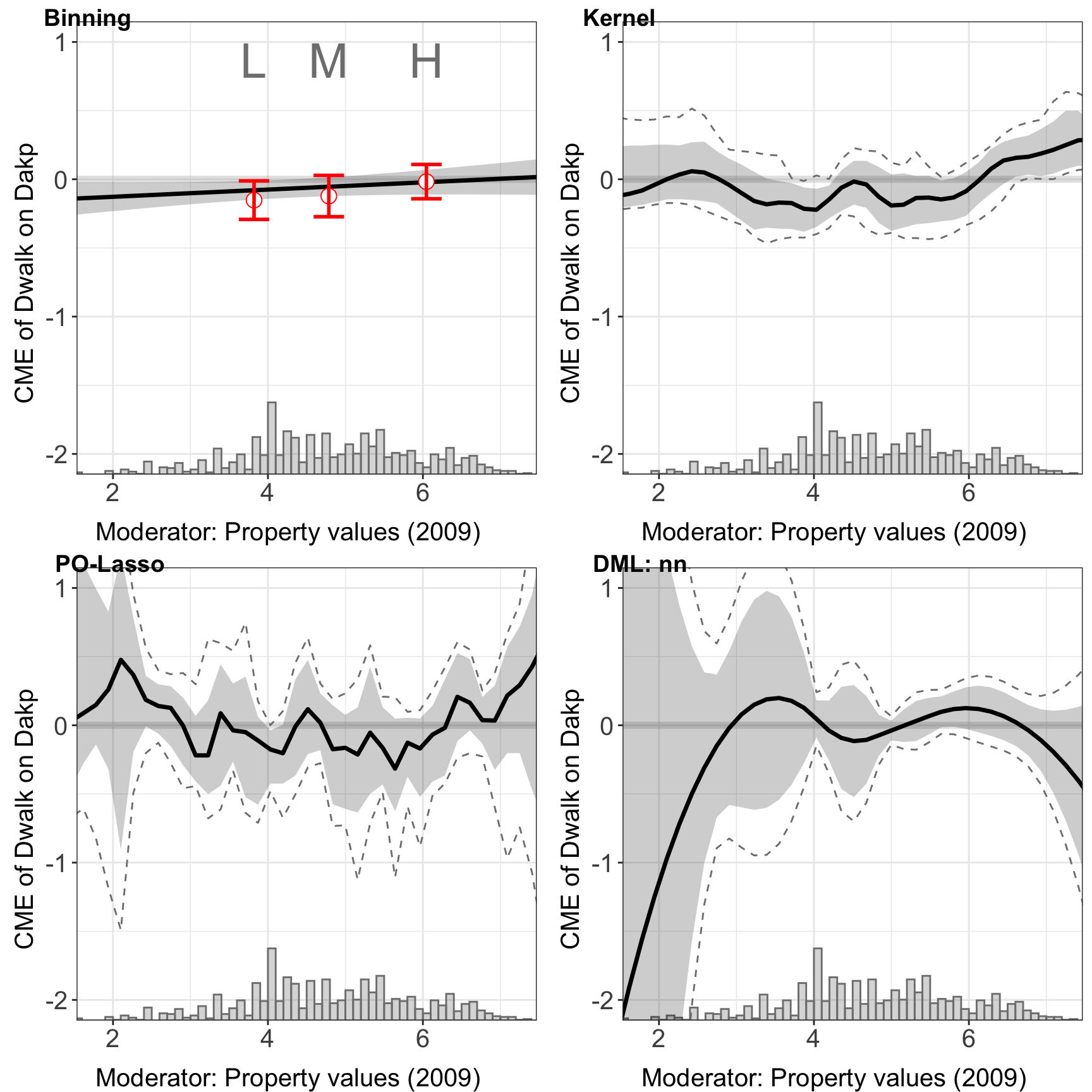
All the advance options, such as first stage model, parameter specification, and cross-validation for parameters are all available in the continuous treatment settings.
Here, we provide another example to explore how selecting different DML parameters affects performance. In this case, we specify the the number of trees in the forest (n_estimators), the minimum number of samples required to split an internal node (min_samples_split), and the the minimum number of samples required to be at a leaf node (min_samples_leaf), using the list param_rf and feed them to the DML estimator. We compare it with the DML estimator using `rf`` as first stage model, but without adjusting parameters.
param_rf <- list(
  n_estimators = as.integer(200),
  min_samples_leaf = as.integer(4)
)

out.dml.rf.para <- interflex(estimator="dml", data = d,
                              Y = Y, D = D, X = X, Z = Z,
                              Ylabel = Ylabel, Dlabel = Dlabel,
                              Xlabel = Xlabel,
                              model.y = "rf", param.y = param_rf,
                              model.t = "rf", param.t = param_rf,
                              main = "Random Forests: Specified Parameters",
                              treat.type = "continuous")
#> Parallel computing: using 8 of 14 available cores.
#> To change: set cores = <n> in interflex().

out.dml.rf<-interflex(estimator="dml", data = d,
                      Y = Y, D = D, X = X, Z = Z,
                      Ylabel = Ylabel, Dlabel = Dlabel,
                      Xlabel = Xlabel,
                      model.y = 'rf', model.t = 'rf',
                      main = "Random Forests: Default")
#> Parallel computing: using 8 of 14 available cores.
#> To change: set cores = <n> in interflex().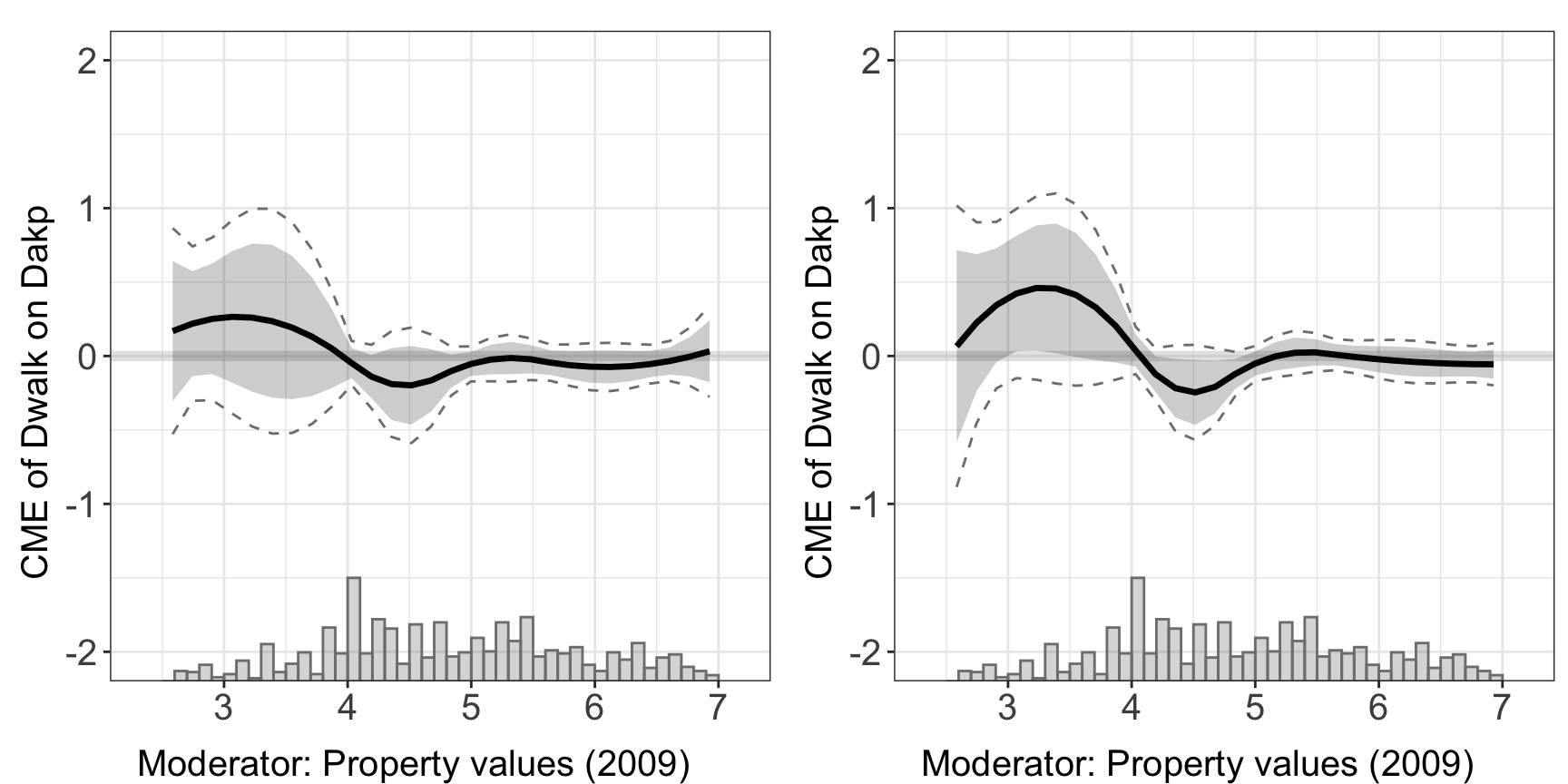
5.4 GATE with discrete moderator
When the moderator \(X\) is discrete, we can estimate Group Average Treatment Effects (GATE) by setting gate = TRUE. This uses the DML orthogonal score to compute average treatment effects within each level of \(X\).
We use the Beiser-McGrath and Bernauer (2024) example with income as a discrete moderator:
data(app_bb2024)
d <- app_bb2024
d <- remove_labels(d)

out.dml.gate <- interflex(estimator = 'dml', data = d,
                          Y = "sup_tax_rebate", D = "treat_type_bin",
                          X = "income",
                          Z = c("leftright", "clim_belief", "resp_age", "female",
                                "employment_f", "highedu", "midedu", "pid_f"),
                          na.rm = TRUE, gate = TRUE,
                          model.y = "linear", model.t = "linear")
#> Parallel computing: using 8 of 14 available cores.
#> To change: set cores = <n> in interflex().
#> Baseline group not specified; choose treat = 0 as the baseline group.out.dml.gate$figure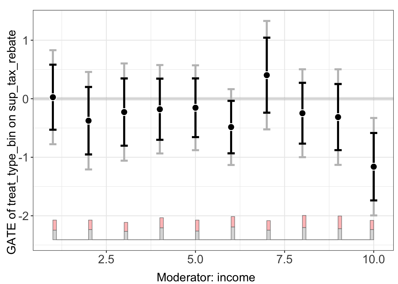
Use plot(..., by.group = TRUE) for separate point estimates and confidence intervals per group:
plot(out.dml.gate, by.group = TRUE)
The g.est field contains the GATE estimates:
out.dml.gate$g.est[[1]]
#>     X          ME        sd lower CI(95%) upper CI(95%) lower uniform CI(95%)
#> 1   1  0.02595273 0.2836119    -0.5299164    0.58182190            -0.7774603
#> 2   2 -0.37539651 0.2940444    -0.9517129    0.20091985            -1.2083624
#> 3   3 -0.22777472 0.2932610    -0.8025558    0.34700635            -1.0585216
#> 4   4 -0.17955564 0.2666809    -0.7022407    0.34312941            -0.9350067
#> 5   5 -0.15412398 0.2559618    -0.6557999    0.34755190            -0.8792099
#> 6   6 -0.48421317 0.2287393    -0.9325339   -0.03589244            -1.1321835
#> 7   7  0.40265551 0.3270960    -0.2384408    1.04375182            -0.5239386
#> 8   8 -0.24766237 0.2651248    -0.7672974    0.27197265            -0.9987052
#> 9   9 -0.31357421 0.2883008    -0.8786333    0.25148490            -1.1302697
#> 10 10 -1.16145656 0.2938840    -1.7374585   -0.58545459            -1.9939681
#>    upper uniform CI(95%)
#> 1              0.8293657
#> 2              0.4575694
#> 3              0.6029722
#> 4              0.5758954
#> 5              0.5709620
#> 6              0.1637571
#> 7              1.3292497
#> 8              0.5033804
#> 9              0.5031213
#> 10            -0.3289451