2 Classic: Basics
In this chapter, we show how to use interflex package to analyze and estimate CME. We begin with visual diagnostics such as subgroup scatterplots, binning plot, and Generalized Additive Models (GAM) plot. We then estimate CME with classic approaches, including linear estimator and kernel estimator; We also show how to use interflex package with binning, linear and kernel estimators when users are interested in extension function, such as multiple treatment arms, fixed effect, prediction, and analyzing differences in treatment effects. We illustrates the implementation details using empirical example, with binary treatment settings and continuous treatment settings.
2.1 Binary treatment
In this example and through out the whole manual, we will use a consistent notation. \(Y\) is the outcome variable, the moderator is \(X\), the covariates are \(Z\).
The example we are using is from Huddy et al. (2015), which explores the effect of the expressive model of partisanship. Drawing on four survey studies, the authors argue that partisan identity drives campaign participation and strong emotional responses to ongoing campaign events. The Conditional Marginal Effect (CME) studied in the paper suggests that strongly identified partisans are more likely to exhibit stronger emotional reactions – such as anger when threatened with electoral loss - compared to those with weaker partisan identities. The variables of interest include:
Outcome variable: level of anger (continuous scale from 0 to 1)
Treatment variable: electoral loss threat or electoral win reassurance (binary yes/no variable)
Moderator Variable: strength of partisan identity (continuous scale from 0 to 1)
d<-app_hma2015

Y = "totangry" ## outcome: anger
D = "threat" ## treatment: threat
X = "pidentity" ## moderator: partisan identity
Z <-  c("issuestr2", "knowledge", "educ","male", "age10")

Ylabel = "Anger"
Dlabel = "Threat"
Xlabel = "Partisanship"

datatable(d)
2.1.1 Diagnostics
2.1.1.1 Raw plots
The first step of the diagnostics is to plot raw data. We supply the function interflex with the variable names of the outcome Y, the treatment D, and the moderator X, and covaraites Z. You can also supply labels for these variables, such as Ylabel, Dlabel, and Xlabel. If you supply a variable name to the weights option, the linear and LOESS fits will be adjusted based on the weights. Note that the correlations between covariates Z and Y are NOT partialled out.
interflex(estimator = "raw",data = d, Y = Y,
                     D = D, X = X, Z = Z,
                     Ylabel = Ylabel, Dlabel = Dlabel,
                     Xlabel = Xlabel,
          main = "Raw plot", ylab = "CME of Threat on Anger")
#> Baseline group not specified; choose treat = 0 as the baseline group.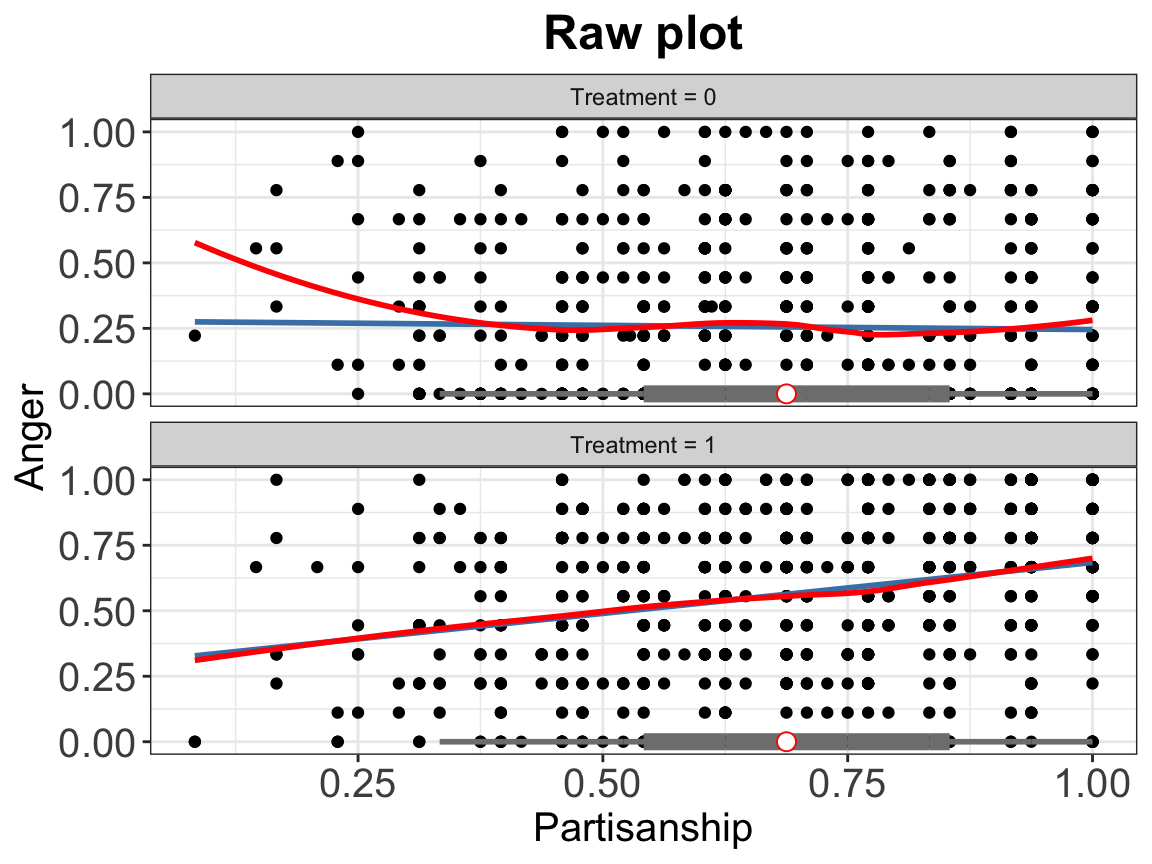
2.1.1.2 Binning plots
The second diagnostic tool is the binning plot. It will discretizes the moderator \(X\) into several bins and create a dummy variable for each bin and picks an evaluation point within each bin, where users want to estimate the CME of \(D\) on \(Y\). The regression terms includes interactions between the bin dummies and the treatment indicator, the bin dummies and the moderator \(X\) minus the evaluation points, as well as the triple interactions.
The histograms at the bottom of the plot depict the distributions of \(X\) across treatment (pink) and control (gray) group. If the CME estimates from the binning estimator sit closely to the estimated CME from the linear estimator, then the Linear Interaction Effect (LIE) assumption likely holds
The nbins option sets the number of bins. The default number of bins is 3, and equal-sized bins are created based on the distribution of the moderator.
bin.out.1 <- interflex(estimator = "binning", data = d,
                 Y = Y,D = D, X = X, Z = Z,
                 Ylabel = Ylabel, Dlabel = Dlabel,
                 Xlabel = Xlabel,
                 main = "Marginal Effects")
#> Baseline group not specified; choose treat = 0 as the baseline group.bin.out.1$figure
For fully moderated model, we includes interactions between each covariate \(Z\) and the bin dummies and the triple interactions. It can reduce biases when the impact of some covariates to the outcome does not take a linear form of moderator \(X\), but sometimes it will also render the estimates unstable when the number of covariates is large.
bin.out.2 <- interflex(estimator = "binning", data = d,
                 Y = Y,D = D, X = X, Z = Z,
                 Ylabel = Ylabel, Dlabel = Dlabel,
                 Xlabel = Xlabel, full.moderate = TRUE,
                 main = "Marginal Effects")
#> Use fully moderated model.
#> Baseline group not specified; choose treat = 0 as the baseline group.bin.out.2$figure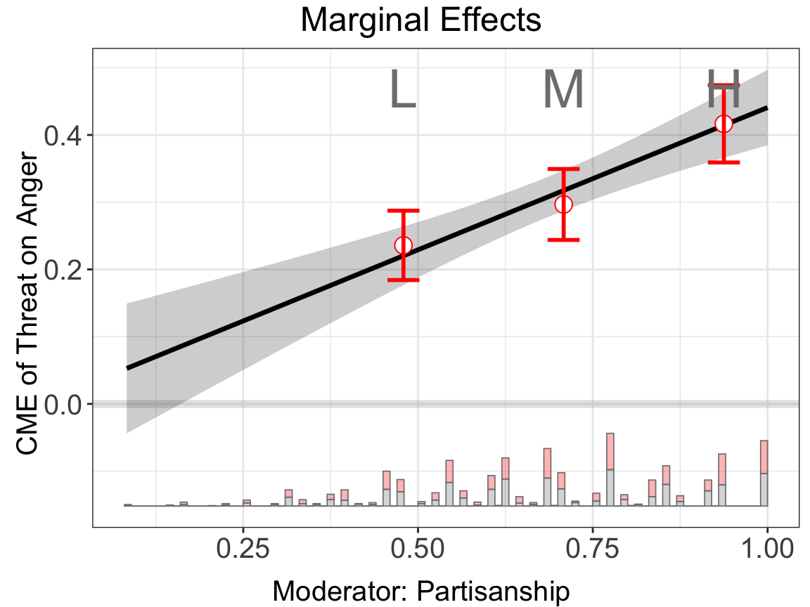
Note that we can customize the cutoff values for the bins, for example, set cutoffs = c(0.25,0.5,0.75,0.9) to create five bins: \([minX, 0.25], (0.25, 0.5], (0.5,0.75], (0.75, 0.9]\) and \((0.9,maxX]\) (supplying N numbers will create N+1 bins). Note that the cutoffs option will override the nbins option if they are incompatible.
bin.out.3$figure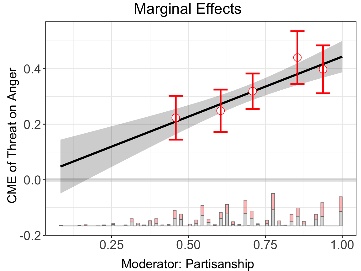
Next, we use Xunif = TRUE to transform the moderator into a uniformly distributed random variable (based on the rank order in values of the orginal moderator) before estimating the CME.
bin.out.4 <- interflex(estimator = "binning", data = d,
                 Y = Y,D = D, X = X, Z = Z,
                 Ylabel = Ylabel, Dlabel = Dlabel,
                 Xlabel = Xlabel, Xunif = TRUE,
                 main = "Marginal Effects")
#> Baseline group not specified; choose treat = 0 as the baseline group.bin.out.4$figure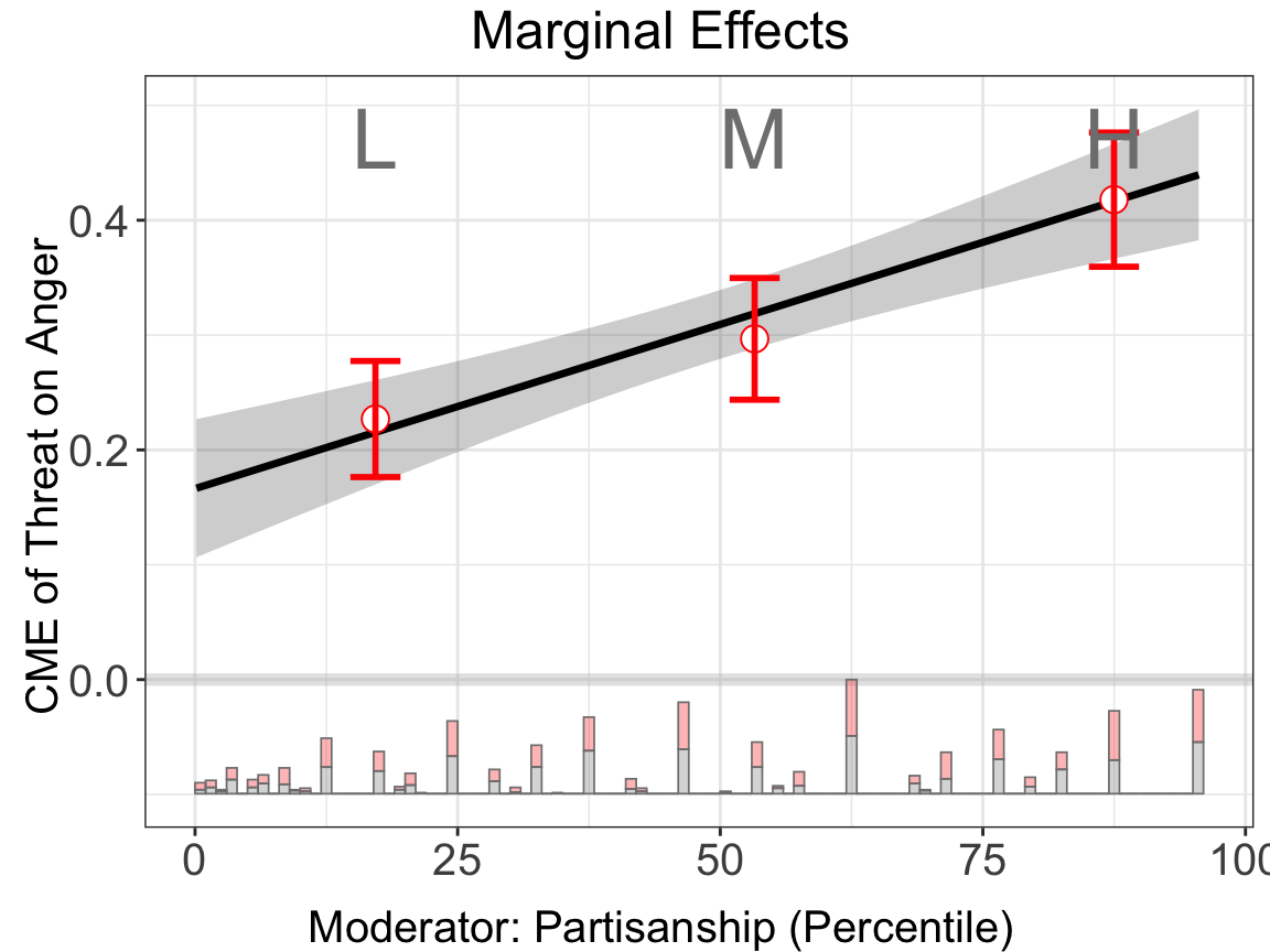
interflex will also automatically report a set of statistics when estimator = "binning", including: (1) the binning estimates and their standard errors and 95% confidence intervals, (2) the percentage of observations within each bin, (3) the L-kurtosis of the moderator, and (4) a Wald test to formally test if we can reject the linear multiplicative interaction model by comparing it with a more flexible model of multiple bins.
The CME plot is stored in object$figure while the estimates and standard errors are stored in object$est.bin (binning). The tests results are stored in object$tests (binning).
print(bin.out.1$tests$p.wald)
#> [1] "0.593"
plot allows users to adjust graphic options without re-estimating the model. The first entry must be a interflex object. Note that we use bin.labs = FALSE to hide the label on the top of each bin and Xdistr = "none to remove the distribution of the moderator (not recommended), or set Xdistr = "density to present the distribution of the moderator with a density plot using option. We use cex.axis and cex.lab to adjust the font sizes of axis numbers and labels. We address all the plotting options in chapter Chapter 7.
plot(bin.out.1, Xdistr = "density", bin.labs = FALSE)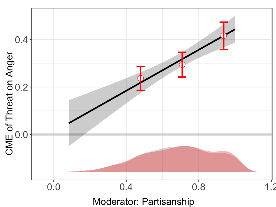
2.1.2 Linear estimator
We first discuss classic approaches to estimating and visualizing the CME. We begin with the linear interaction model, which remains widely used in social science research.
Estimation. If we want to deploy the linear estimator, we can set estimator = "linear". This method estimates CME with multiplicative interaction model. When the option full.moderate is set to TRUE, interaction terms between the moderator \(X\) and each covariate \(Z\) will enter the model, which is the case in Blackwell and Olson (2020). This extension in some cases can reduce the bias of the original model.
Uncertainty estimation. Depending on vartype, the estimator computes standard errors and confidence intervals in three ways simu, delta, and bootstrap. The option vartype = "simu" draws from a multivariate normal distribution multiple times, vartype = "delta" uses a matrix derivatives to approximate the variance.
We report the uniform/simultaneous confidence interval along with pointwise confidence interval. Pointwise CI is estimated by default, and is depicted by gray ribbon; Uniform CI is estimated when setting vartype = "bootstrap" and vartype = "delta", as depicted by the dashed lines.
Note that the variance-covariance matrix of coefficients used by the delta method or the simulation method by default is the robust standard error matrix estimated from the regression. Users can also choose homoscedastic or cluster standard error by specifying the option vcov.type. There are four options for the choice of the vcov estimator: vcov.type = "homoscedastic", "robust", "cluster", and "pcse". The default option is "robust".
linear.out.1 <- interflex(estimator = "linear", data = d,
                 Y = Y,D = D, X = X, Z = Z,
                 Ylabel = Ylabel, Dlabel = Dlabel,
                 Xlabel = Xlabel, vartype = "bootstrap",
                 main = "Linear model")
#> Parallel computing: using 8 of 14 available cores.
#> To change: set cores = <n> in interflex().
#> Baseline group not specified; choose treat = 0 as the baseline group.

linear.out.2 <- interflex(estimator = "linear", data = d,
                 Y = Y,D = D, X = X, Z = Z,
                 Ylabel = Ylabel, Dlabel = Dlabel,
                 Xlabel = Xlabel,
                 vartype = "bootstrap", full.moderate = TRUE,
                 main = "Fully Moderated Linear model")
#> Parallel computing: using 8 of 14 available cores.
#> To change: set cores = <n> in interflex().
#> Use fully moderated model.
#> Baseline group not specified; choose treat = 0 as the baseline group.ggarrange(linear.out.1$figure, linear.out.2$figure)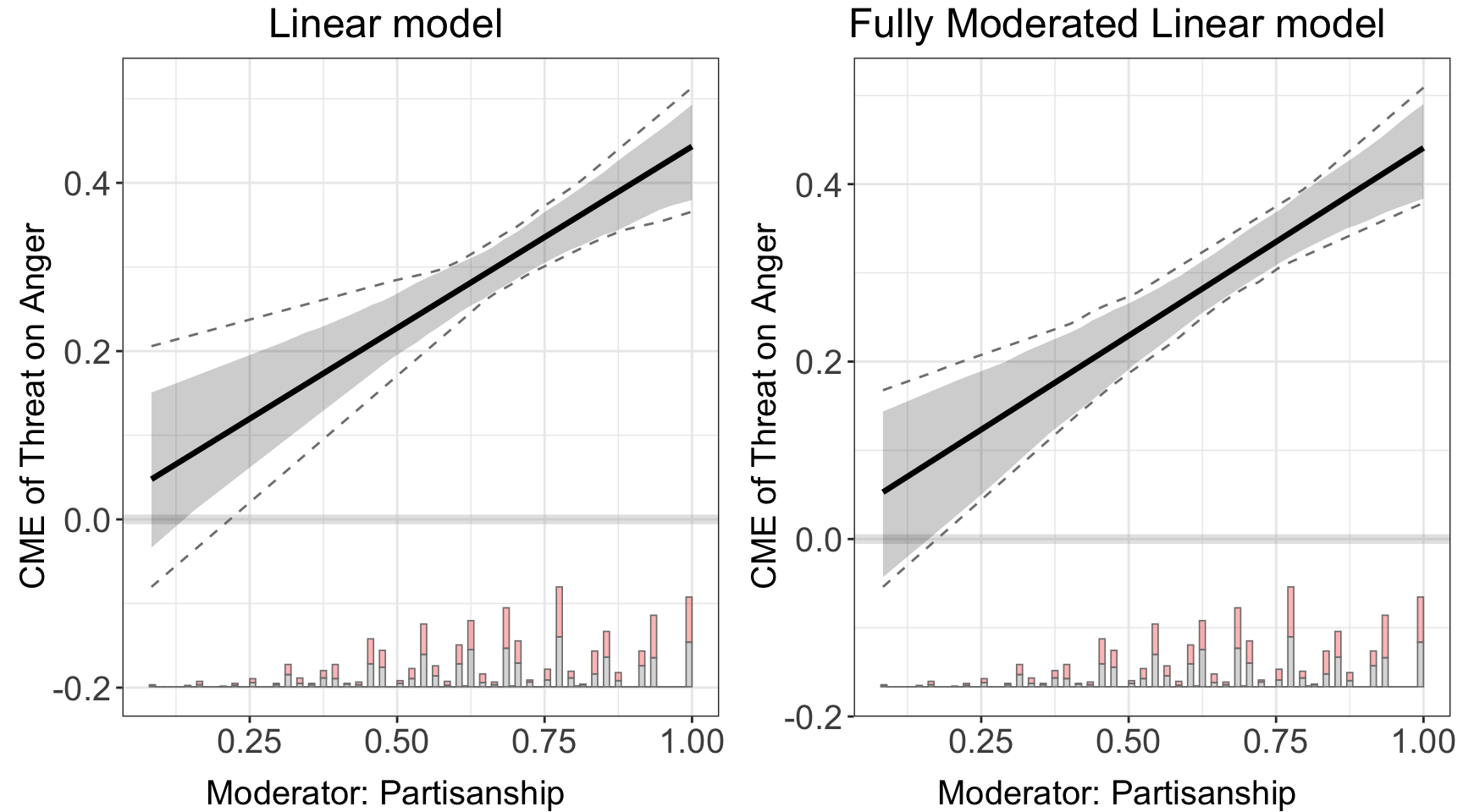
Parallel computing will speed up both cross-validation and uncertainty estimation significantly. We recommend that users manually set the number of cores using the cores option. If this is not supplied or is NULL, interflex will automatically select the smaller of 8 and the number of usable system cores minus 2, to prevent excessive use of system resources.
Results. The CME plot is stored in out$figure while the estimates and standard errors are stored in out$est.lin
head(linear.out.1$est.lin$`1`)
#>               X         TE         sd lower CI(95%) upper CI(95%)
#> [1,] 0.08333334 0.04769277 0.05002516 -0.0336936442     0.1507600
#> [2,] 0.10204082 0.05576608 0.04861109 -0.0222450239     0.1556115
#> [3,] 0.12074830 0.06383938 0.04720118 -0.0107964036     0.1605962
#> [4,] 0.13945578 0.07191268 0.04579583  0.0006522167     0.1656284
#> [5,] 0.15816327 0.07998599 0.04439546  0.0118912919     0.1706607
#> [6,] 0.17687075 0.08805929 0.04300056  0.0220114880     0.1756929
#>      lower uniform CI(95%) upper uniform CI(95%)
#> [1,]           -0.08026810             0.2058570
#> [2,]           -0.06900170             0.2094027
#> [3,]           -0.05773531             0.2129484
#> [4,]           -0.04646891             0.2164941
#> [5,]           -0.03520252             0.2200399
#> [6,]           -0.02393612             0.2235856
2.1.3 Uniform confidence intervals
By default, interflex reports both pointwise and uniform confidence intervals (CIs) when vartype = "bootstrap". The pointwise CI covers the true CME at each individual value of \(X\) with 95% probability, but it does not guarantee simultaneous coverage across all values of \(X\). The uniform CI, by contrast, provides a confidence band that covers the entire CME curve simultaneously with 95% probability. This is analogous to the distinction between individual and family-wise error rates in multiple testing.
Uniform CIs are wider than pointwise CIs. They are important when making statements about the shape of the CME curve as a whole — for example, “the treatment effect is positive for all values of \(X > 0\)” requires the uniform band to be above zero for the entire region of \(X > 0\), not just each pointwise interval. In the plots, pointwise CIs appear as shaded ribbons and uniform CIs appear as dashed lines.
The bootstrapped uniform CI works by finding the narrowest band that achieves simultaneous 95% coverage across all \(k\) evaluation points. With \(N\) bootstrap draws, the smallest resolvable tail probability is approximately \(1/N\), and the algorithm improves on the Bonferroni correction only when \(N > 2k/\alpha\). For the default \(\alpha = 0.05\):
| Evaluation points (\(k\)) | Minimum nboots
|
|---|---|
| 10 | 400 |
| 20 | 800 |
| 50 (default) | 2,000 |
| 100 | 4,000 |
With the default nboots = 200, the algorithm falls back to the conservative Bonferroni correction for most cases. We recommend setting nboots = 2000 or higher when uniform CIs are of interest.
Here we demonstrate the linear estimator with vartype = "bootstrap" and nboots = 2000 to obtain proper uniform CIs:
linear.uni <- interflex(estimator = "linear", data = d,
                 Y = Y, D = D, X = X, Z = Z,
                 Ylabel = Ylabel, Dlabel = Dlabel,
                 Xlabel = Xlabel, vartype = "bootstrap",
                 nboots = 2000, main = "With Uniform CI (nboots = 2000)")
#> Parallel computing: using 8 of 14 available cores.
#> To change: set cores = <n> in interflex().
#> Baseline group not specified; choose treat = 0 as the baseline group.linear.uni$figure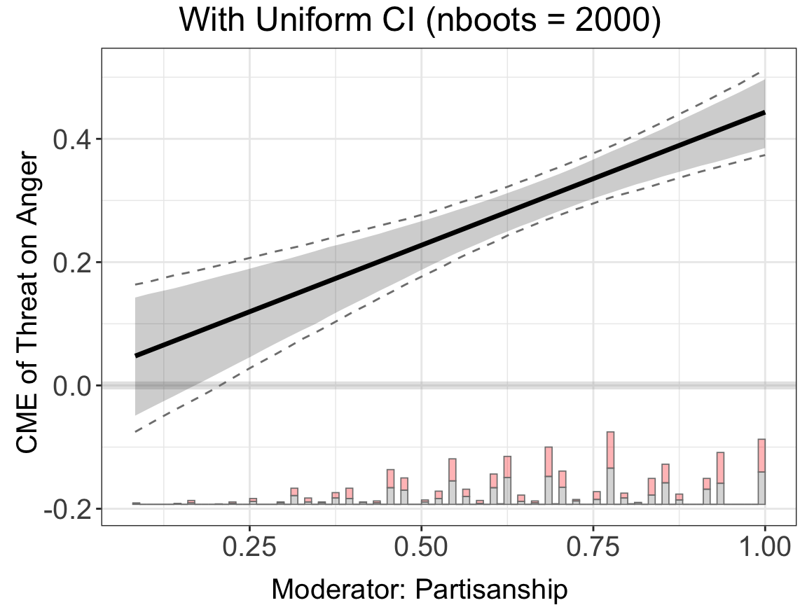
To turn off uniform CIs (e.g., to reduce visual clutter or when only pointwise inference is needed), set show.uniform.CI = FALSE in either the estimation or plotting call:
linear.nouni <- interflex(estimator = "linear", data = d,
                 Y = Y, D = D, X = X, Z = Z,
                 Ylabel = Ylabel, Dlabel = Dlabel,
                 Xlabel = Xlabel, vartype = "bootstrap",
                 nboots = 2000,
                 show.uniform.CI = FALSE, main = "Without Uniform CI")
#> Parallel computing: using 8 of 14 available cores.
#> To change: set cores = <n> in interflex().
#> Baseline group not specified; choose treat = 0 as the baseline group.linear.nouni$figure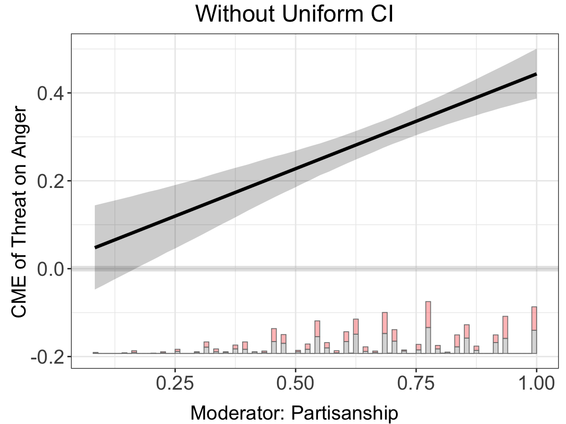
You can also hide uniform CIs at the plotting stage without re-estimating:
plot(linear.uni, show.uniform.CI = FALSE)2.1.4 Kernel estimator
To relax functional form assumptions, we then explore the kernel estimator proposed by Hainmueller et al. (2019).
Estimation. Similar to other estimator, to deploy the kernel estimator, we can set estimator = "kernel". We also provide full.moderate option, allowing moderator \(X\) and each covariate \(Z\) to fully interact.
Uncertainty estimation. Kernel estimator computes standard errors in two ways: delta and bootstrap. Uniform CI is estimated when setting vartype = "bootstrap".
When the standard errors are produced bootstrapping, we can adjust the number of bootstrap iterations using the nboots option, with the default being 200 (set nboots = 2000 or higher for proper uniform CIs; see the note above). The grid option can either be an integer, which specifies the number of bandwidths to be cross-validated, or a vector of candidate bandwidths – the default is grid = 20. We can also specify a clustered group structure by using the cl option, in which case a block bootstrap procedure will be performed.
The left panel uses the default settings for the kernel estimator; the right panel use fully interacted model, with nboots = 400, and we set the estimator to choose bandwidths from c(0,1,2,3)
kernel.out.1 <- interflex(estimator = "kernel",
                          data = d,
                 Y = Y,D = D, X = X, Z = Z,
                 Ylabel = Ylabel, Dlabel = Dlabel,
                 Xlabel = Xlabel,
                 vartype = "bootstrap", bw = 0.916,
                 main = "Kernel model")
#> Parallel computing: using 8 of 14 available cores.
#> To change: set cores = <n> in interflex().
#> Baseline group not specified; choose treat = 0 as the baseline group.
#> Number of evaluation points:50


kernel.out.2 <- interflex(estimator = "kernel",
                          data = d,
                 Y = Y,D = D, X = X, Z = Z,
                 Ylabel = Ylabel, Dlabel = Dlabel,
                 Xlabel = Xlabel,
                 vartype = "bootstrap", grid = c(0,1,2,3), full.moderate = TRUE,
                 main = "Fully Moderated Kernel model")
#> Parallel computing: using 8 of 14 available cores.
#> To change: set cores = <n> in interflex().
#> Use fully moderated model.
#> Baseline group not specified; choose treat = 0 as the baseline group.
#> Cross-validating bandwidth ...
#> Optimal bw=3.
#> Number of evaluation points:50ggarrange(kernel.out.1$figure, kernel.out.2$figure)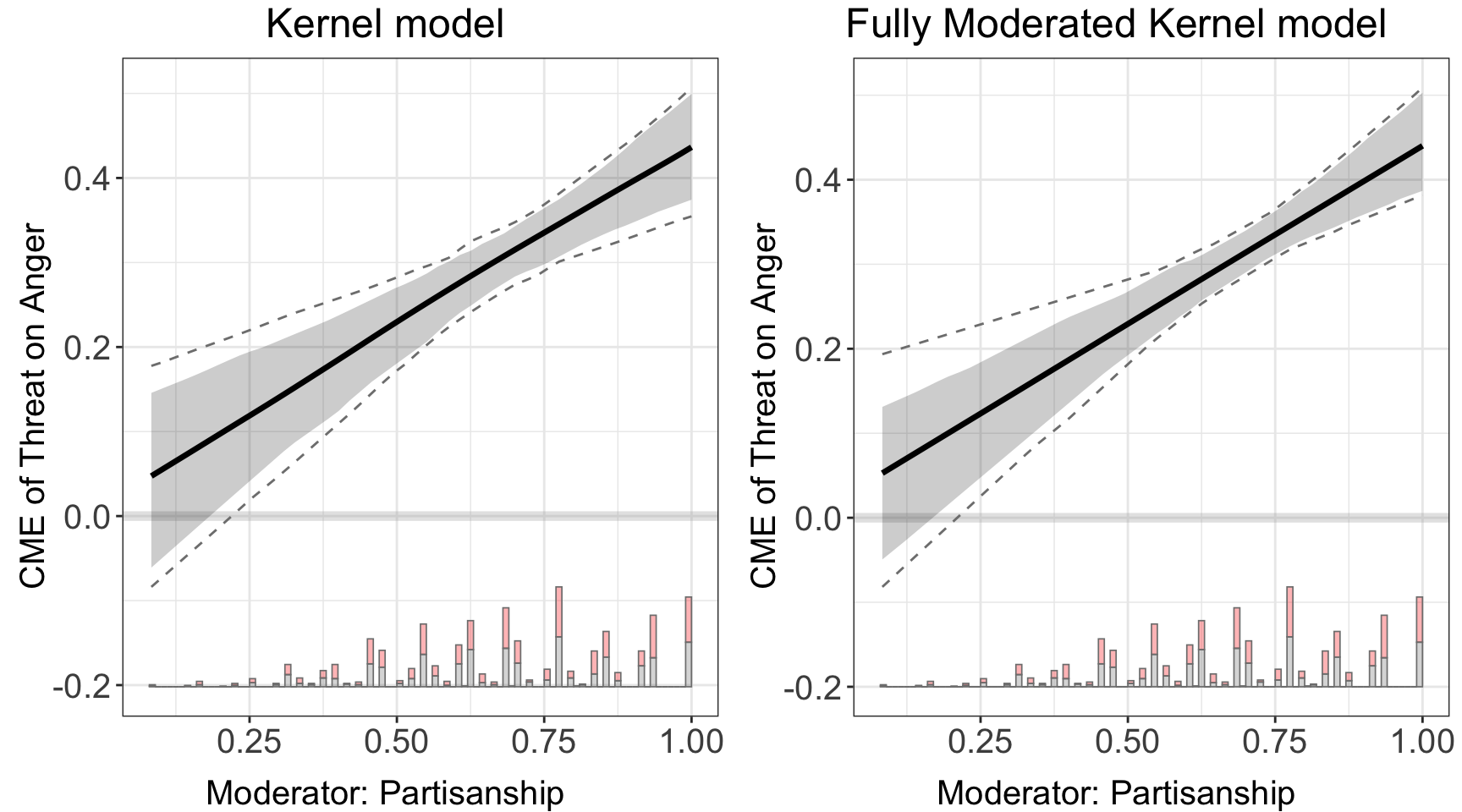
Bandwidth selection. We use adaptive bandwidth selection in interflex. This means that the bandwidth will be smaller in regions where there are more data and larger in regions where there are few data points, based on the moderator \(X\). When adaptive bandwidth is being used, bw refers to the bandwidth applied in the region with the highest density of observations.
Even with an optimized algorithm, the bootstrap procedure for large datasets can be slow. We incorporate parallel computing, parallel=TRUE, to speed it up. You can choose the number of cores to be used for parallel computing; otherwise the program will detect the number of logical cores in your computer and use as many cores as possible (warning: this will significantly slow down your computer!).
If you specify a bandwidth manually, for example, by setting bw = 1, the cross-validation step will be skipped.
cat("1. Runtime with parallel computing for Bandwidth selection:\n")
#> 1. Runtime with parallel computing for Bandwidth selection:
runtime_parallel <- system.time({
  kernel.out.parallel <- interflex(estimator = "kernel", data = d,
                                   Y = Y, D = D, X = X, Z = Z,
                                   Ylabel = Ylabel, Dlabel = Dlabel,
                                   Xlabel = Xlabel,
                                   vartype = "bootstrap", parallel = TRUE,
                                   main = "Linear model")
})
#> Parallel computing: using 8 of 14 available cores.
#> To change: set cores = <n> in interflex().
#> Baseline group not specified; choose treat = 0 as the baseline group.
#> Cross-validating bandwidth ...
#> Optimal bw=0.9167.
#> Number of evaluation points:50
cat("User Time: ", runtime_parallel[1], " seconds\n")
#> User Time:  7.331  seconds
cat("System Time: ", runtime_parallel[2], " seconds\n")
#> System Time:  0.483  seconds
cat("Elapsed Time: ", runtime_parallel[3], " seconds\n\n")
#> Elapsed Time:  18.853  seconds

cat("2. Runtime with user-specified Bandwidth selection:\n")
#> 2. Runtime with user-specified Bandwidth selection:
runtime_user_bandwidth <- system.time({
  kernel.out.user_bandwidth <- interflex(estimator = "kernel", data = d,
                                         Y = Y, D = D, X = X, Z = Z,
                                         Ylabel = Ylabel, Dlabel = Dlabel,
                                         Xlabel = Xlabel,
                                         bw = 0.9,
                                         main = "Linear model")
})
#> Baseline group not specified; choose treat = 0 as the baseline group.
#> Number of evaluation points:50
cat("User Time: ", runtime_user_bandwidth[1], " seconds\n")
#> User Time:  0.412  seconds
cat("System Time: ", runtime_user_bandwidth[2], " seconds\n")
#> System Time:  0.01  seconds
cat("Elapsed Time: ", runtime_user_bandwidth[3], " seconds\n")
#> Elapsed Time:  0.421  seconds
Results. The estimation results, including pointwise and uniform confidence intervals, are included in est.kernel.
head(kernel.out.1$est.kernel$`1`)
#>               X         TE         sd lower CI(95%) upper CI(95%)
#> [1,] 0.08333334 0.04732898 0.05340622  -0.060997774     0.1457363
#> [2,] 0.10204082 0.05532476 0.05191087  -0.049494668     0.1510136
#> [3,] 0.12074830 0.06331515 0.05042394  -0.037992472     0.1562312
#> [4,] 0.13945578 0.07129443 0.04894463  -0.026499679     0.1614532
#> [5,] 0.15816327 0.07931711 0.04747660  -0.015009896     0.1668755
#> [6,] 0.17687075 0.08736605 0.04601356  -0.003519963     0.1725302
#>      lower uniform CI(95%) upper uniform CI(95%)
#> [1,]           -0.08380802             0.1776929
#> [2,]           -0.07232664             0.1819727
#> [3,]           -0.06086035             0.1868661
#> [4,]           -0.04938939             0.1917582
#> [5,]           -0.03793331             0.1965798
#> [6,]           -0.02647701             0.2012807
The results of cross-validation are saved in CV.output.
head(kernel.out.1$CV.output)
#> NULL
2.2 Continuous treatment
Adiguzel et al. (2023) examines the impact of incumbent’s public health provision on electoral outcomes. The authors use a reform in Turkey that significantly altered the geographic distribution of health clinics. The authors find that reduced congestion levels significantly increased the AKP’s vote share, especially in poorer communities which exhibited a more substantial response to the improvements in health care access. The variables of interest are:
- Outcome: Change in the vote share for the incumbent AKP party (continuous, \(\in [-33.9, 39.5]\))
- Treatment: Change in congestion (continuous, \(\in [-28.8, 20.8]\)); congestion is measured by the number of patients per doctor at the nearest clinic, with lower congestion indicating improved service quality
- Moderator: Logarithm of median property value (continuous, \(\in[-0.2, 7.7]\))
data(app_adiguzel2023)
d<-app_adiguzel2023
d<-remove_labels(d)
d<-as.data.frame(d)
main<-"Adiguzel2023a"
D="Dwalk_3"
Y="Dakp_3"
X="lograyic09"

Z=c('Duniversity_3', 'Dodr_3', 'Dydr_3', 'Dpopulation_3', 'Dhospital_pri_3', 'Dhospital_pub_3')

Dlabel<-"Dwalk"
Ylabel<-"Dakp"
Xlabel<-"Property values (2009)"

#datatable(d)
2.2.1 Diagnostics
2.2.1.1 Raw plots
Similar to the binary treatment settings, we can plot the subgroup scatter plot as first step of diagnostics:
interflex(estimator = "raw",data = d, Y = Y,
                     D = D, X = X, Z = Z,
                     Ylabel = Ylabel, Dlabel = Dlabel,
                     Xlabel = Xlabel,
          main = "Raw plot", ylab = "CME")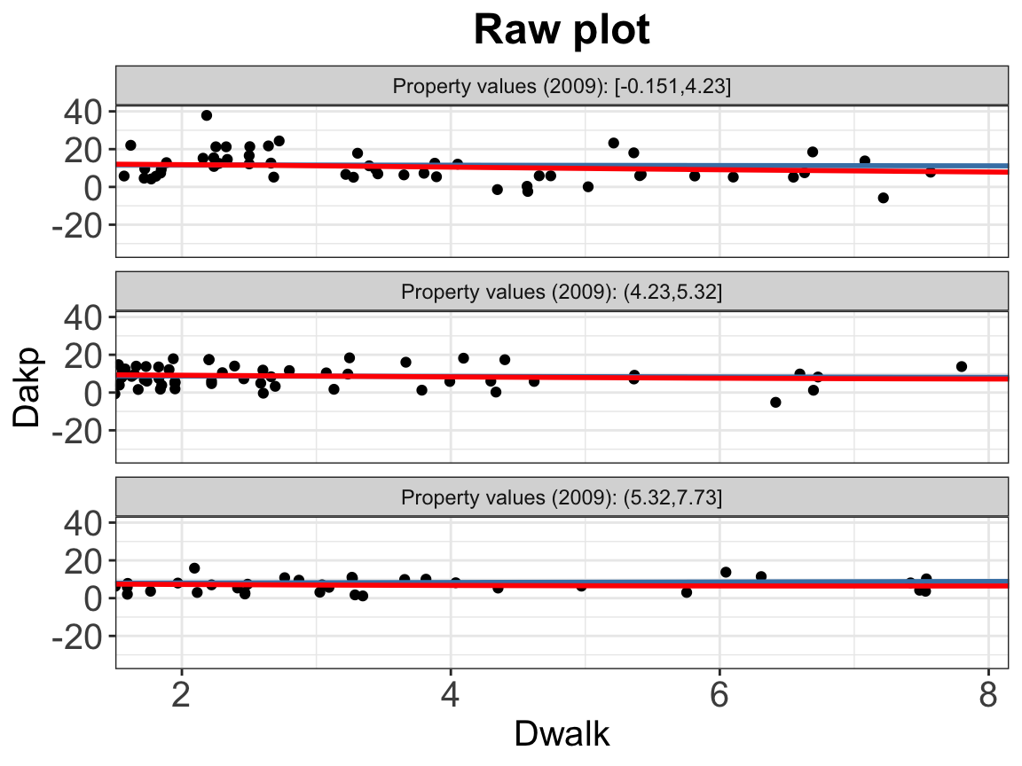
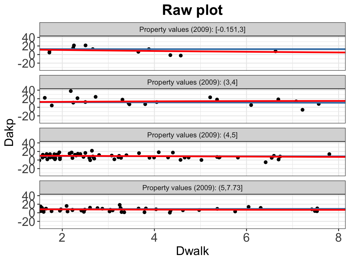
Instead of grouping by treatment status, the scatter plot carves \(X\) into 3 quantile‐based bins by default. You can supply your own number of bins by setting the cutoff =. Supplying \(N\) numbers will create \(N+1\) bins.
2.2.1.2 Binning plots
Similar to the binary treatment case, we can also use binning plot for diagnosis.
bin.out.1<-interflex(estimator = "binning",data = d, Y = Y,
                     D = D, X = X, Z = Z,
                     Ylabel = Ylabel, Dlabel = Dlabel,
                     Xlabel = Xlabel, cutoff = cut_bins,
main = "Binning plot", ylab = "CME")bin.out.1$figure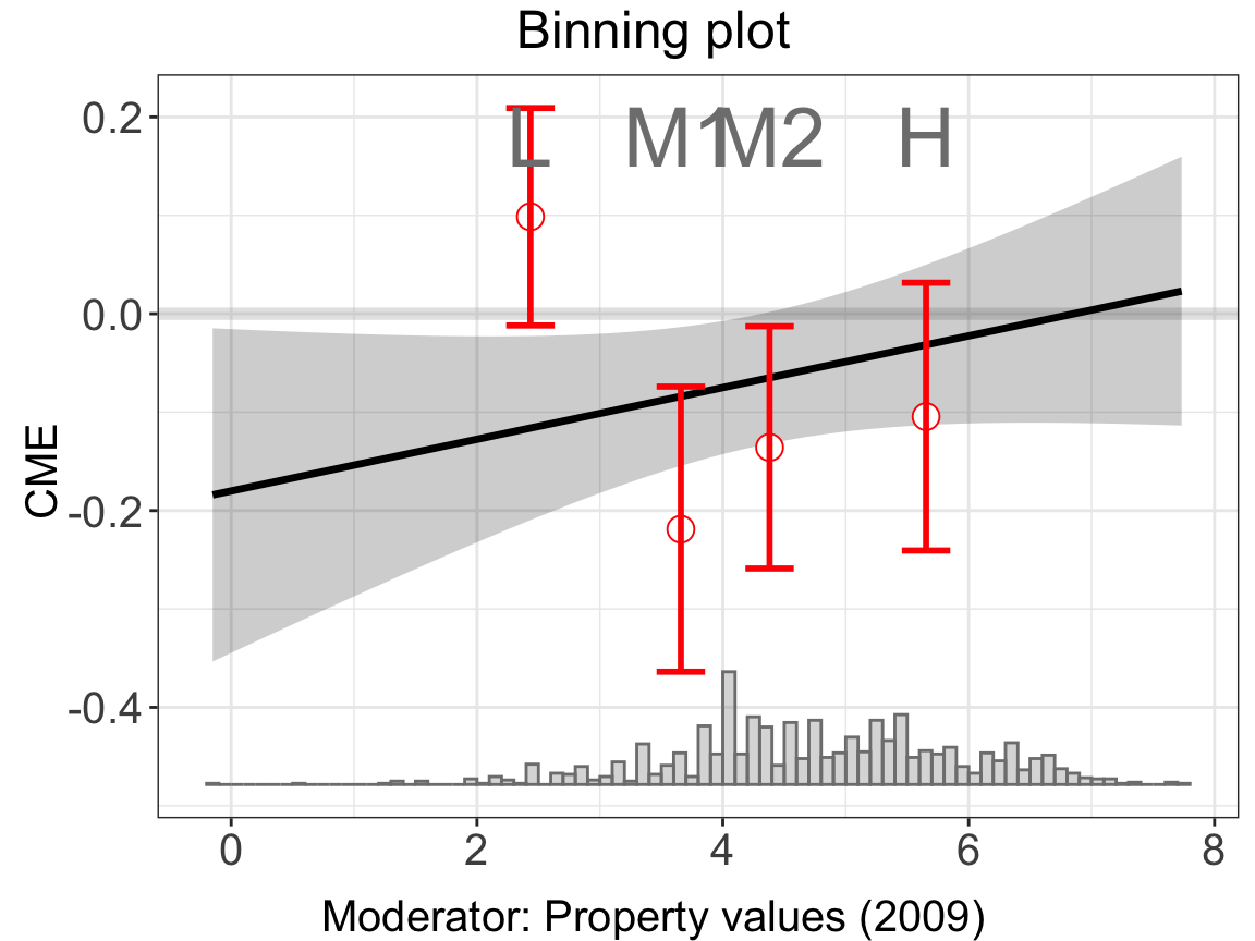
Because the treatment group is not binary, the histograms at the bottom of the plot simply depict the distribution of \(X\), not differentiating by treatment status.
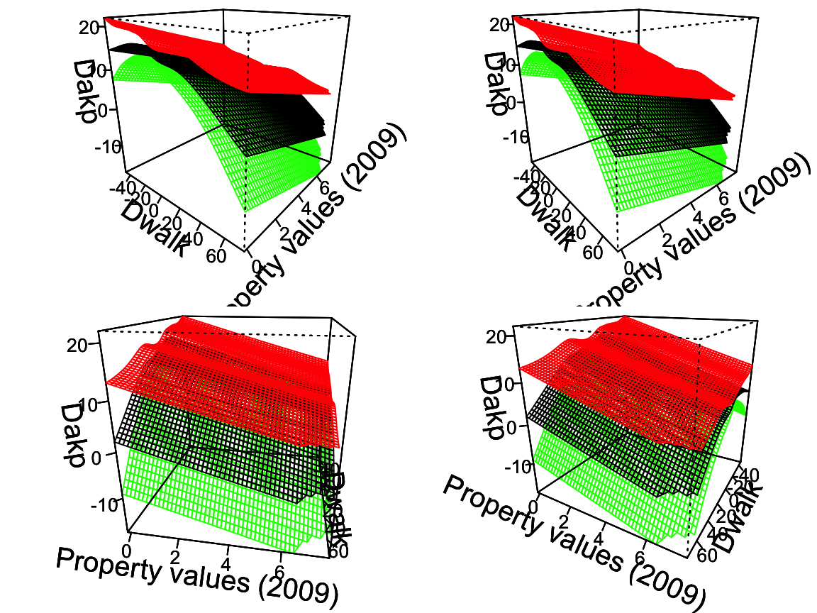
2.2.1.3 GAM plots
For the continuous treatment case, we can draw a Generalized Additive Model (GAM) plot.
interflex(estimator = "gam",data = d, Y = Y,
                     D = D, X = X, Z = Z,
                     Ylabel = Ylabel, Dlabel = Dlabel,
                     Xlabel = Xlabel, show.uniform.CI = FALSE,
          main = "GAM plot", ylab = "CME")
You can manipulate the angle of each of the four plots by setting angle with your own value of theta, which change the azimuth (horizontal rotation) angle in degrees. The default angle is c(30, 100,-30,-120).
#>
#> Family: gaussian
#> Link function: identity
#>
#> Formula:
#> Dakp_3 ~ s(Dwalk_3, lograyic09, k = 10) + Duniversity_3 + Dodr_3 +
#>     Dydr_3 + Dpopulation_3 + Dhospital_pri_3 + Dhospital_pub_3
#>
#> Estimated degrees of freedom:
#> 5.61  total = 12.61
#>
#> GCV score: 40.48669
2.2.2 Linear estimator
We illustrate the code implementation using an empirical example with a continuous treatment. Note that the coding approach is essentially the same for both continuous and binary treatments.
linear.out.1 <- interflex(estimator = "linear", data = d,
                 Y = Y,D = D, X = X, Z = Z,
                 Ylabel = Ylabel, Dlabel = Dlabel,
                 Xlabel = Xlabel,
                 main = "Linear model")

linear.out.2 <- interflex(estimator = "linear", data = d,
                 Y = Y,D = D, X = X, Z = Z,
                 Ylabel = Ylabel, Dlabel = Dlabel,
                 Xlabel = Xlabel, full.moderate = TRUE,
                 main = "Fully Moderated Linear model")
#> Use fully moderated model.ggarrange(linear.out.1$figure, linear.out.2$figure)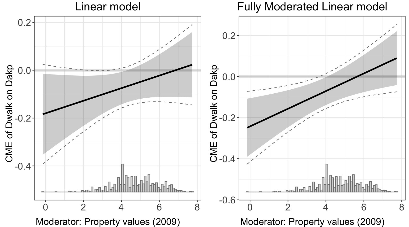
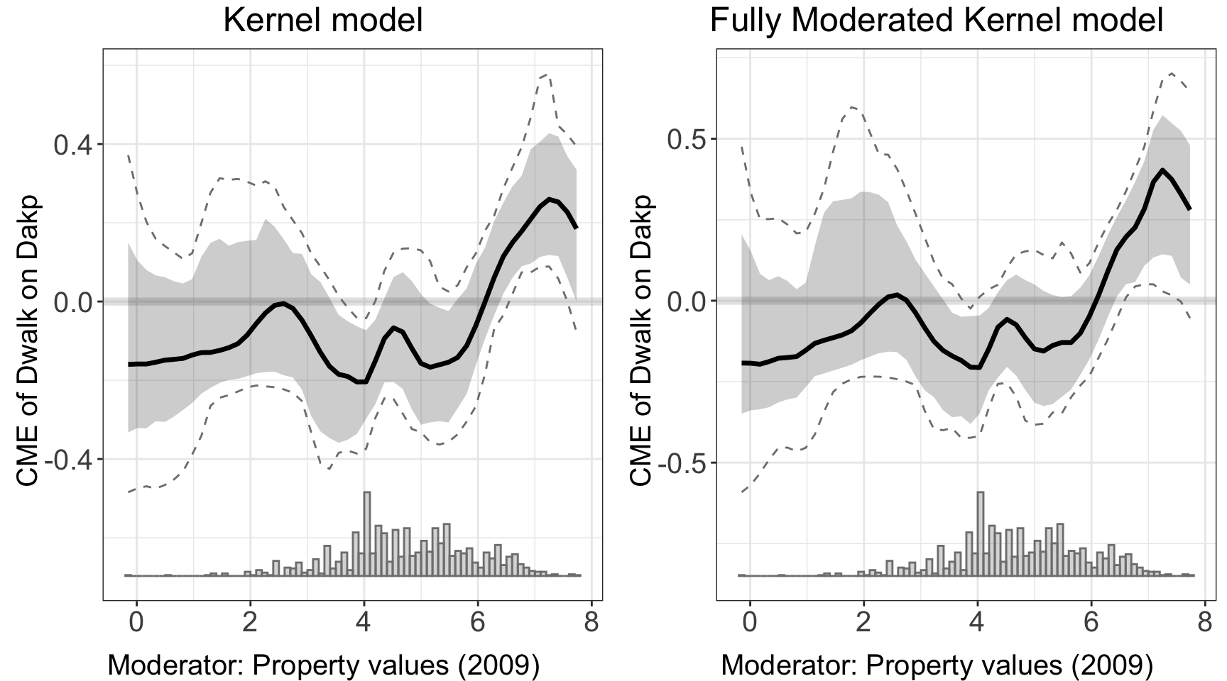
2.2.3 Kernel estimator
We can deploy kernel estimator with the same syntax.
kernel.out.1 <- interflex(estimator = "kernel",
                          data = d,
                 Y = Y,D = D, X = X, Z = Z,
                 Ylabel = Ylabel, Dlabel = Dlabel,
                 Xlabel = Xlabel,
                 vartype = "bootstrap",
                 main = "Kernel model")
#> Parallel computing: using 8 of 14 available cores.
#> To change: set cores = <n> in interflex().
#> Cross-validating bandwidth ...
#> Optimal bw=1.0004.
#> Number of evaluation points:50

kernel.out.2 <- interflex(estimator = "kernel",
                          data = d,
                 Y = Y,D = D, X = X, Z = Z,
                 Ylabel = Ylabel, Dlabel = Dlabel,
                 Xlabel = Xlabel,
                 vartype = "bootstrap", grid = c(0,1,2,3), full.moderate = TRUE,
                 main = "Fully Moderated Kernel model")
#> Parallel computing: using 8 of 14 available cores.
#> To change: set cores = <n> in interflex().
#> Use fully moderated model.
#> Cross-validating bandwidth ...
#> Optimal bw=1.
#> Number of evaluation points:50ggarrange(kernel.out.1$figure, kernel.out.2$figure)