data(br2017, package = "sconjoint")
dim(br2017)
[1] 32000 35This chapter applies the structural estimator to a tax-plan conjoint experiment from Ballard-Rosa, Martin, and Scheve (2017). Respondents evaluate pairs of hypothetical income tax plans varying on six marginal tax rates (one per income bracket) plus a revenue impact indicator, and select the plan they prefer. The bundled br2017 is the paper’s full analysis frame (2,000 respondents, 32,000 rows), so the quantities below reproduce the empirical results reported in the manuscript.
What makes this dataset unique among the bundled examples is that every attribute is numeric (continuous). There are no factor attributes — the six bracket rates are percentages and the revenue score is a centered integer scale. This showcases how sconjoint handles all-numeric attribute designs.
data(br2017, package = "sconjoint")
dim(br2017)[1] 32000 35str(br2017, list.len = 12)'data.frame': 32000 obs. of 35 variables:
$ respondent : chr "177191531" "177191531" "177191531" "177191531" ...
$ task : int 1 1 2 2 3 3 4 4 5 5 ...
$ profile : int 1 2 1 2 1 2 1 2 1 2 ...
$ choice : int 1 0 1 0 1 0 1 0 1 0 ...
$ rate_L10 : num 5 0 15 15 25 25 15 25 5 25 ...
$ rate_10_35 : num 25 35 25 15 15 35 35 35 25 25 ...
$ rate_35_85 : num 35 5 5 15 15 35 35 5 5 35 ...
$ rate_85_175 : num 25 15 25 15 35 5 15 25 25 15 ...
$ rate_175_375 : num 15 5 25 35 35 25 25 25 15 5 ...
$ rate_375P : num 5 45 25 5 55 5 45 55 15 25 ...
$ revenue_score : num 0 1 0 -1 1 2 2 2 -1 2 ...
$ resp_pid7 : num 5 5 5 5 5 5 5 5 5 5 ...
[list output truncated]Each respondent contributes eight forced-choice tasks with two tax-plan profiles each (16 rows per respondent). The fit conditions on 23 respondent-level moderators (\(\mathbf Z_i\)): demographics (age_std, female, educ_std, race_white, income_std, children), partisanship and ideology (pid7_std, conserv_ideo), economic attitudes and beliefs (ineq_averse, work_vs_luck, taxes_harm_econ, hardwork, high_econ_know, govt_serv, gov_assist), economic position (employed_ft, gen_mobile, future_mobile, hardship, risk_averse), and engagement/competence (newsint, numeracy, trust). The raw seven-point party identification is also retained as a convenience column, resp_pid7 (1 = strong Democrat to 7 = strong Republican), which we use below to split respondents by party. It is not part of the moderator set (pid7_std is its standardized counterpart).
Every attribute here is continuous, with the tax rates encoded as percentage points (0–55). The paper handles this with the varref Stage-2 prior and a low variance floor (varref_floor = 1e-3) on the raw rates, rather than the default score-based map_c5 prior. We follow the paper’s recipe exactly here. Coefficients are in “logit utility per percentage point” units.
fit_br <- scfit(
  choice ~ rate_L10 + rate_10_35 + rate_35_85 + rate_85_175 +
           rate_175_375 + rate_375P + revenue_score |
           age_std + female + pid7_std + educ_std + race_white +
           income_std + ineq_averse + work_vs_luck + taxes_harm_econ +
           hardwork + high_econ_know + employed_ft + conserv_ideo +
           govt_serv + newsint + numeracy + gen_mobile + future_mobile +
           gov_assist + risk_averse + hardship + children + trust,
  data         = br2017,
  respondent   = "respondent",
  task         = "task",
  profile      = "profile",
  K            = 10L,
  seed         = 42L,
  stage2       = "varref",
  varref_floor = 1e-3,
  parallel     = TRUE,
  n_cores      = 10L
)
summary(fit_br)
sc_fit summary
Call: scfit(formula = choice ~ rate_L10 + rate_10_35 + rate_35_85 +
rate_85_175 + rate_175_375 + rate_375P + revenue_score |
age_std + female + pid7_std + educ_std + race_white + income_std +
ineq_averse + work_vs_luck + taxes_harm_econ + hardwork +
high_econ_know + employed_ft + conserv_ideo + govt_serv +
newsint + numeracy + gen_mobile + future_mobile + gov_assist +
risk_averse + hardship + children + trust, data = br2017,
respondent = "respondent", task = "task", profile = "profile",
K = 10L, seed = 42L, parallel = TRUE, n_cores = 10L, stage2 = "varref",
varref_floor = 0.001)
2000 respondents | 16000 observations | K = 10 folds
hidden = 32-32-16 | epochs = 1000 | seed = 42 | device = cpu | parallel (10 cores)
Coefficients (DML, respondent-clustered SE):
estimate std_error z_value p_value ci_lo ci_hi
rate_L10 -0.064453 0.003721 -17.321 3.282e-67 -0.071746 -0.0571596
rate_10_35 -0.043598 0.005388 -8.091 5.903e-16 -0.054158 -0.0330369
rate_35_85 -0.024687 0.002945 -8.382 5.225e-17 -0.030460 -0.0189140
rate_85_175 -0.002946 0.001980 -1.488 1.368e-01 -0.006826 0.0009344
rate_175_375 0.010018 0.001687 5.937 2.895e-09 0.006711 0.0133251
rate_375P 0.018695 0.002020 9.256 2.124e-20 0.014736 0.0226539
revenue_score 0.139588 0.047156 2.960 3.075e-03 0.047163 0.2320127
DML/iid SE ratio (mean): 1.063
Stage 2: varref | mean(sigma_prior) = 0.001This is the paper’s exact recipe, run on the corrected bracket-5 data (the distributed file mis-stored the 45% level of the $175-375k bracket; see ?br2017) with varref_floor = 1e-3. The estimates below therefore reproduce the manuscript’s reported numbers.
stage2 = "varref" for continuous attributes?
The default map_c5 Stage-2 prior is calibrated assuming \(\mathrm{Var}(\Delta X_k) \approx 1\) (true for factor dummies under typical randomization). BR’s tax rates span 0–50 percentage points, so the score-based prior becomes loose and the MAP solver leaves per-respondent estimates with extreme tails. The paper instead uses the varref prior — \(0.5\cdot\mathrm{Var}_i(\hat\beta_{\text{ens},i,k})\), floored at varref_floor — on the raw rates. The low floor matters: the prior 0.01 default over-shrinks continuous coefficients and badly degrades recovery of individual progressivity, so continuous designs use varref_floor = 1e-3 (the paper’s setting). An alternative is normalize_deltaX = TRUE with the default map_c5 prior, which standardizes \(\Delta X\) internally; see the Advanced options chapter. For factor-dummy designs (SW, GS) neither is needed.
plot(fit_br, "loss_trace")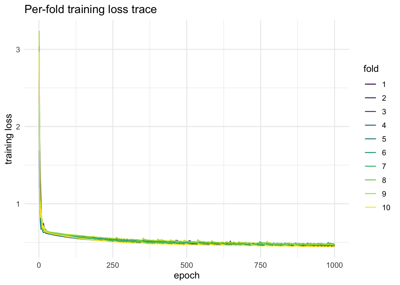
DML coefficients per attribute, on the logit scale, with respondent- clustered SEs. With numeric attributes the coefficient is “logit utility per unit of the attribute” (per percentage-point of the rate, or per unit of the centered revenue indicator).
The population pattern is the paper’s main result: a steep progressive structure in the bracket rates. The average voter dislikes higher rates on low brackets (\(\hat\theta_{<\$10k} \approx -0.06\)) and mildly favors higher rates on the top bracket (\(\hat\theta_{>\$375k} \approx +0.02\)), with the coefficients rising monotonically across brackets and crossing zero around the \(85-175k bracket. The **revenue-impact** coefficient is **weak-positive** (\)$, \(p < 0.01\), 95% CI \([0.05, 0.23]\)): voters prefer plans that raise more revenue, but it is the least important of the seven attributes.
plot_amce(fit_br, groups = br_groups, labels = br_labels)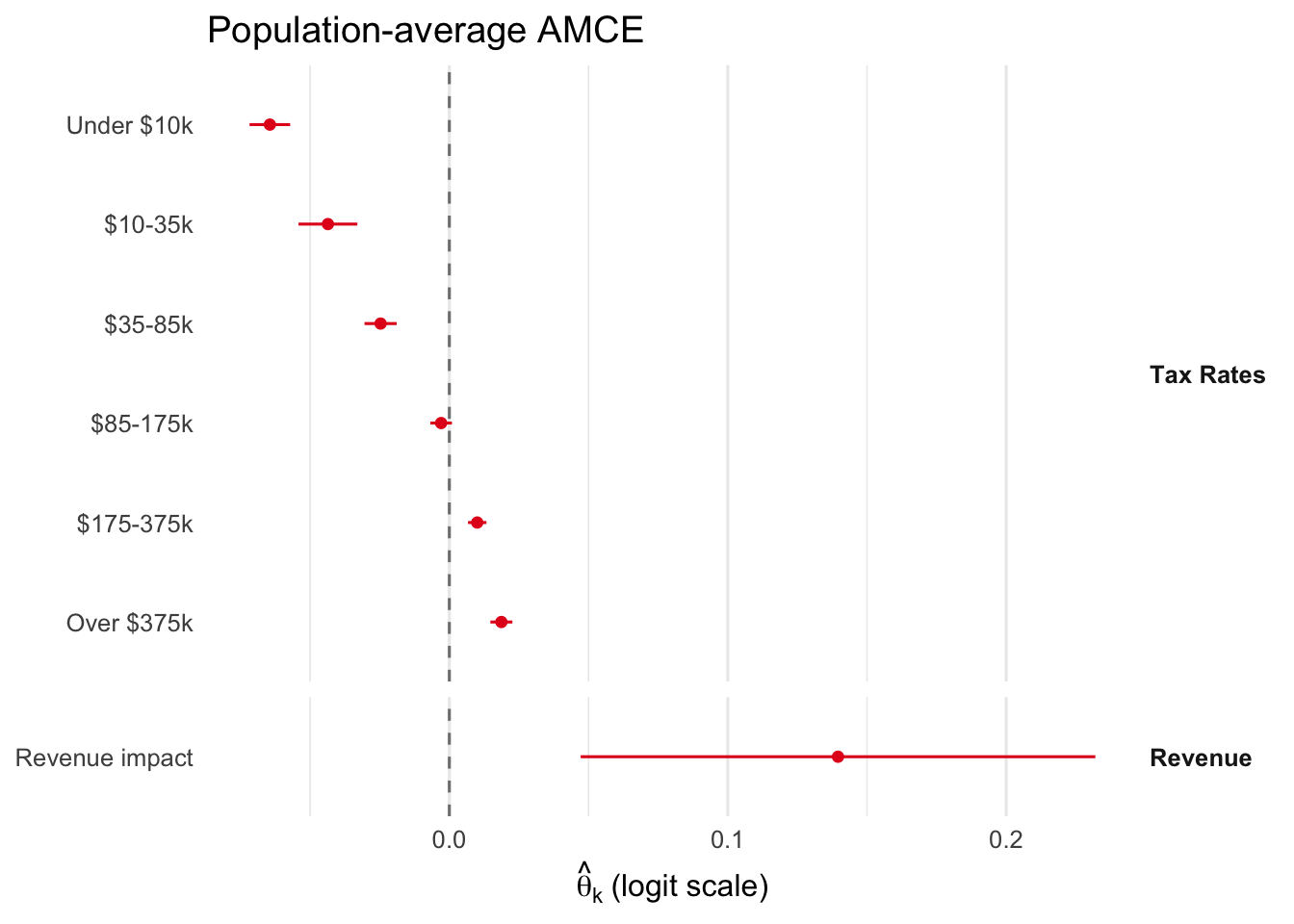
For continuous attributes the AME is “average effect on Pr(choice) per unit of the attribute”. Overlay the structural and LPM versions on the probability scale.
ame_struct <- sc_average(fit_br, scale = "probability")
ame_df     <- ame_struct$estimate; ame_df$source <- "Structural AME"
lpm        <- sc_baseline_lpm(fit_br)
amce_df    <- data.frame(
  dummy_name = names(stats::coef(lpm)),
  estimate   = unname(stats::coef(lpm)),
  se         = sqrt(diag(stats::vcov(lpm))),
  source     = "LPM AMCE",
  stringsAsFactors = FALSE
)
amce_df$ci_lo <- amce_df$estimate - 1.96 * amce_df$se
amce_df$ci_hi <- amce_df$estimate + 1.96 * amce_df$se
df_both <- rbind(
  ame_df[, c("dummy_name", "estimate", "se", "ci_lo", "ci_hi", "source")],
  amce_df[, c("dummy_name", "estimate", "se", "ci_lo", "ci_hi", "source")]
)
df_both$label <- ifelse(df_both$dummy_name %in% names(br_labels),
                        br_labels[df_both$dummy_name],
                        df_both$dummy_name)
df_both$label <- factor(df_both$label, levels = rev(unname(br_labels)))
df_both$group <- br_groups[df_both$dummy_name]
df_both$group <- factor(df_both$group, levels = unique(br_groups))

ggplot(df_both, aes(x = estimate, y = label, color = source)) +
  geom_vline(xintercept = 0, linetype = "dashed", color = "gray50") +
  geom_pointrange(aes(xmin = ci_lo, xmax = ci_hi),
                  position = position_dodge(width = 0.5),
                  size = 0.35, fatten = 2) +
  scale_color_manual(values = c("Structural AME" = "#2166AC",
                                "LPM AMCE"        = "#B2182B")) +
  facet_grid(group ~ ., scales = "free_y", space = "free_y") +
  labs(x = "Effect on Pr(choice)",
       y = NULL, color = NULL,
       title = "Structural AME vs LPM AMCE (probability scale)") +
  theme_minimal(base_size = 11) +
  theme(legend.position = "bottom",
        strip.text.y    = element_text(angle = 0, hjust = 0, face = "bold"))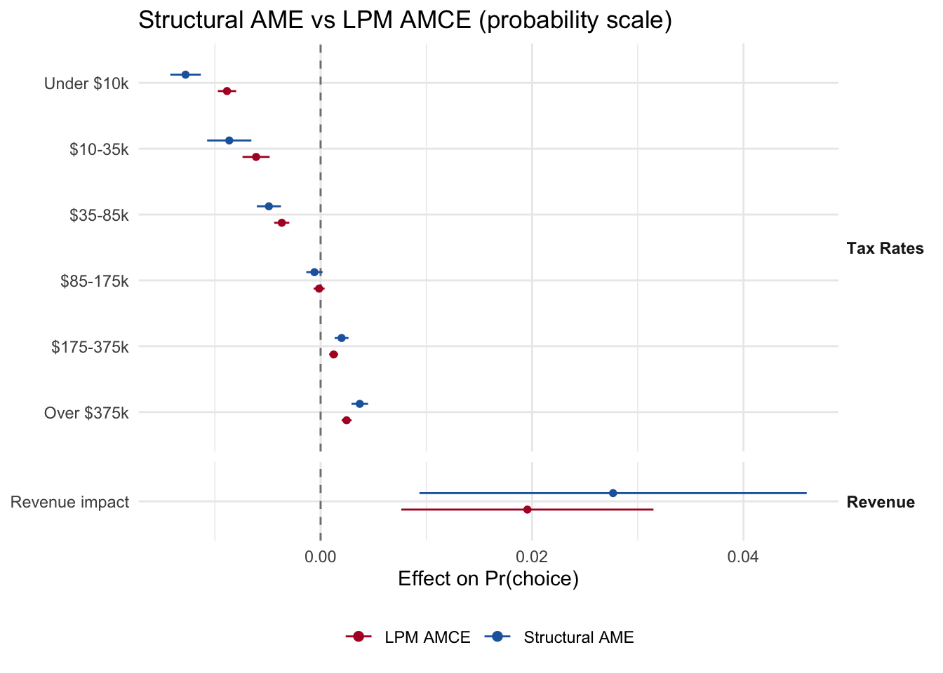
On the paper’s reporting convention (the effect of a one-percentage-point rate increase evaluated at a 50% baseline, \(\hat\theta_k \times 25\)), the bottom-bracket and top-bracket AMEs are about \(-1.6\) and \(+0.5\) percentage points of choice probability. Voters punish a rate hike on the poorest bracket more than threefold as hard as they reward an equal-sized hike on the richest bracket — a sharp asymmetry that the homogeneous AMCE reproduces but cannot attribute to any subgroup.
Ridgeline densities of \(\hat\beta_k(\mathbf Z_i)\) per attribute across respondents. With the varref prior (the fit above) the MAP refinement is properly scaled — the hybrid view shows clean per-respondent distributions for every bracket.
plot(fit_br, "beta_ridgelines", groups = br_groups, labels = br_labels)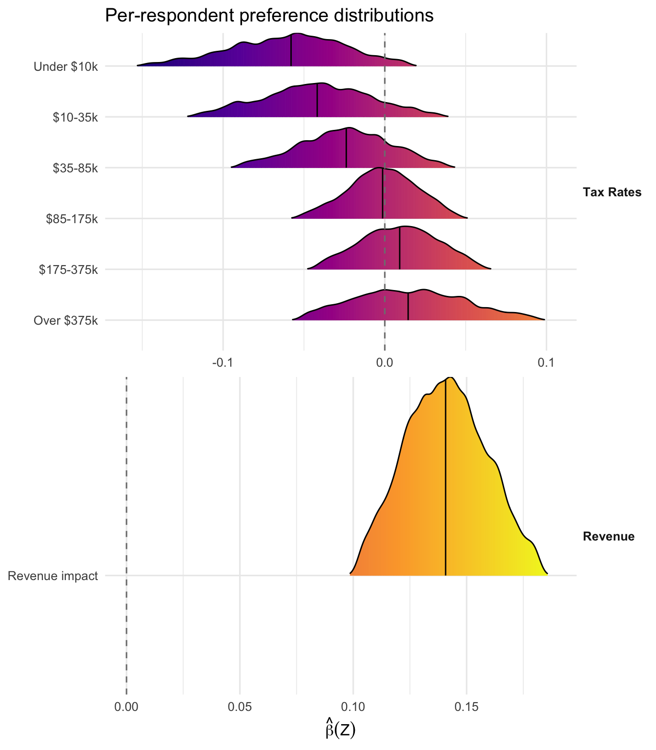
For continuous attributes the paper’s importance share weights each respondent’s squared coefficient by the population variance of the attribute’s design level set (e.g. c(0, 5, 15, 25) for the bottom bracket). This is design = "levels", passing the six brackets’ level sets plus the revenue scale; the default design = "design_variance" gives essentially the same shares here.
br_levels <- list(
  rate_L10     = c(0, 5, 15, 25),  rate_10_35   = c(5, 15, 25, 35),
  rate_35_85   = c(5, 15, 25, 35), rate_85_175  = c(5, 15, 25, 35),
  rate_175_375 = c(5, 15, 25, 35, 45),
  rate_375P    = c(5, 15, 25, 35, 45, 55),
  revenue_score = c(-2, -1, 0, 1, 2)
)
sc_importance(fit_br, design = "levels", levels = br_levels)
sc_quantity: importance
estimate: data.frame with 7 rows
attribute share se ci_lo ci_hi
rate_L10 0.25795 0.0043830 0.24936 0.26654
rate_10_35 0.20829 0.0039189 0.20061 0.21597
rate_35_85 0.12041 0.0030685 0.11440 0.12642
rate_85_175 0.05010 0.0017757 0.04662 0.05358
rate_175_375 0.09140 0.0024536 0.08659 0.09620
rate_375P 0.23445 0.0049980 0.22465 0.24424
revenue_score 0.03741 0.0008194 0.03580 0.03901plot_importance(fit_br, labels = c(
rate_L10 = "Under $10k", rate_10_35 = "$10-35k",
rate_35_85 = "$35-85k", rate_85_175 = "$85-175k",
rate_175_375 = "$175-375k", rate_375P = "Over $375k",
revenue_score = "Revenue"
))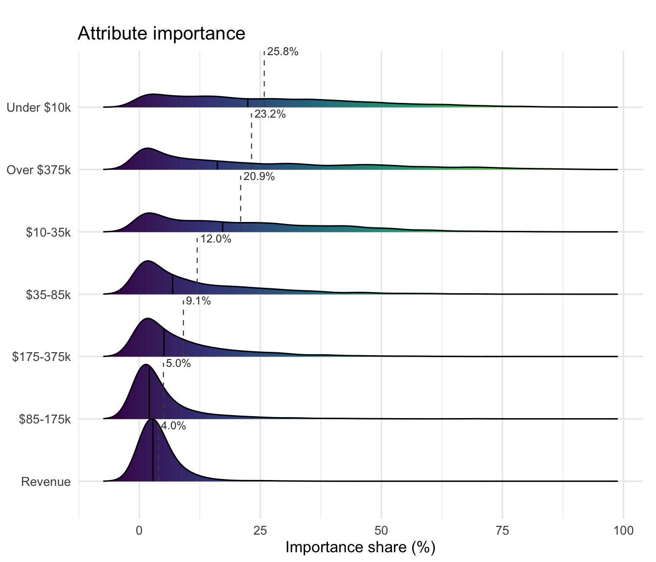
The importance shares differ sharply by party, which is the paper’s second main finding. Among Democrats, the top bracket (>$375k) is the single most important attribute (about 29%) and the low bracket ($10-35k) matters much less (about 16%); among Republicans the ranking inverts, with the $10-35k bracket the most important (about 26%) and the top bracket far less so (about 18%). The $35-85k bracket is roughly twice as important to Republicans (about 18%) as to Democrats (about 8%). In short, Democrats weight what the rich pay, Republicans weight what the middle and working class pay.
imp_by_party <- function(sel) {
  ip <- sc_importance(fit_br, design = "levels", levels = br_levels,
                      subgroup = sel)
  setNames(round(100 * ip$estimate$share, 1), ip$estimate$attribute)
}
## raw 7-point party id, aligned to the fit's task rows
pid7_resp <- tapply(br2017$resp_pid7, as.character(br2017$respondent),
                    function(x) x[1])
pid7_row  <- pid7_resp[as.character(fit_br$respondent_id)]
pid7_row[pid7_row >= 8] <- 4          # "not sure / other" -> Independent
rbind(
  Democrat    = imp_by_party(pid7_row <= 3),
  Independent = imp_by_party(pid7_row == 4),
  Republican  = imp_by_party(pid7_row >= 5)
)
rate_L10 rate_10_35 rate_35_85 rate_85_175 rate_175_375 rate_375P
Democrat 27.7 15.9 8.5 4.4 10.5 29.2
Independent 27.4 22.9 11.0 5.7 9.5 19.6
Republican 22.0 26.1 17.6 5.4 7.1 18.4
revenue_score
Democrat 3.8
Independent 3.9
Republican 3.5sc_direction_intensity(fit_br)sc_quantity_bivariate: direction_intensity
-- direction --
sc_quantity: direction
estimate: data.frame with 7 rows
dummy_name d se_d ci_lo_d ci_hi_d
rate_L10 -0.888 0.01028 -0.90816 -0.867842
rate_10_35 -0.746 0.01489 -0.77519 -0.716807
rate_35_85 -0.582 0.01819 -0.61765 -0.546352
rate_85_175 -0.048 0.02234 -0.09179 -0.004213
rate_175_375 0.261 0.02159 0.21868 0.303318
rate_375P 0.288 0.02142 0.24602 0.329980
revenue_score 1.000 0.00000 1.00000 1.000000
-- intensity --
sc_quantity: intensity
estimate: data.frame with 7 rows
dummy_name u se_u ci_lo_u ci_hi_u
rate_L10 0.06303 0.0008603 0.06135 0.06472
rate_10_35 0.04744 0.0007047 0.04605 0.04882
rate_35_85 0.03230 0.0005379 0.03124 0.03335
rate_85_175 0.01894 0.0003414 0.01827 0.01961
rate_175_375 0.02238 0.0003801 0.02164 0.02313
rate_375P 0.03257 0.0005844 0.03142 0.03372
revenue_score 0.14092 0.0004508 0.14003 0.14180plot_fraction(fit_br, groups = br_groups, labels = br_labels)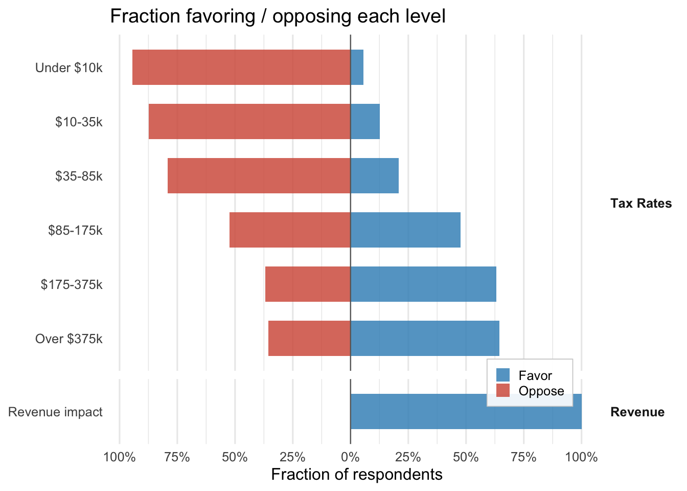
sc_heterogeneity_test(fit_br, adjust = "bh")sc_quantity: heterogeneity_test
estimate: data.frame with 7 rows
dummy_name var_beta se_var t_stat p_value p_adjusted sig
rate_L10 0.0017220 7.771e-05 22.16 4.270e-109 4.270e-109 ***
rate_10_35 0.0014580 5.137e-05 28.39 1.530e-177 3.570e-177 ***
rate_35_85 0.0010273 3.673e-05 27.97 1.765e-172 3.089e-172 ***
rate_85_175 0.0005893 2.124e-05 27.75 9.162e-170 1.283e-169 ***
rate_175_375 0.0007062 2.465e-05 28.65 7.292e-181 2.552e-180 ***
rate_375P 0.0014912 5.491e-05 27.16 9.910e-163 1.156e-162 ***
revenue_score 0.0004063 1.309e-05 31.05 5.682e-212 3.978e-211 ***plot_hetero(fit_br, groups = br_groups, labels = br_labels)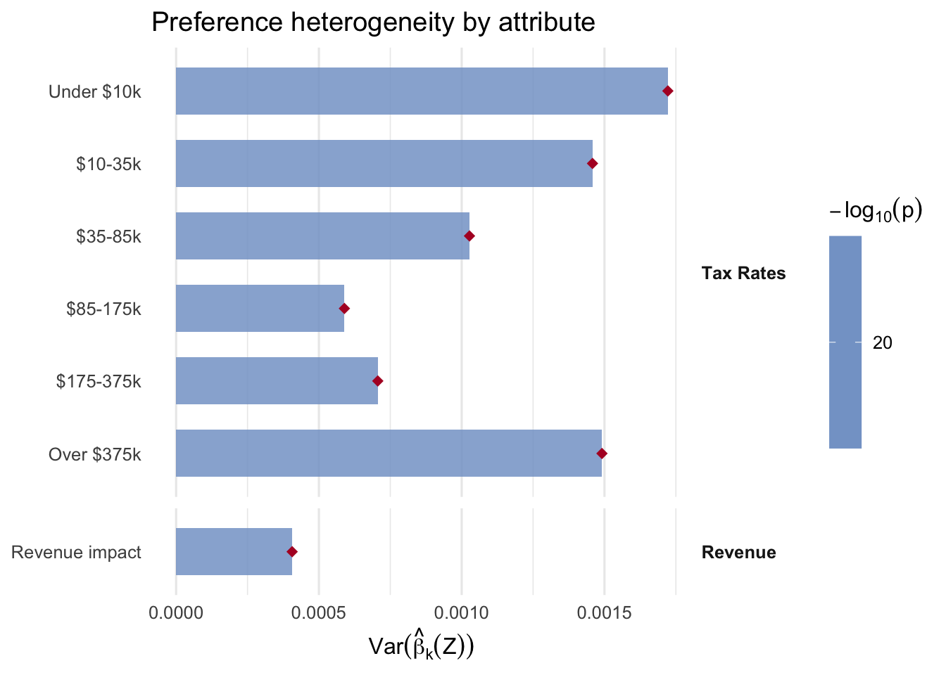
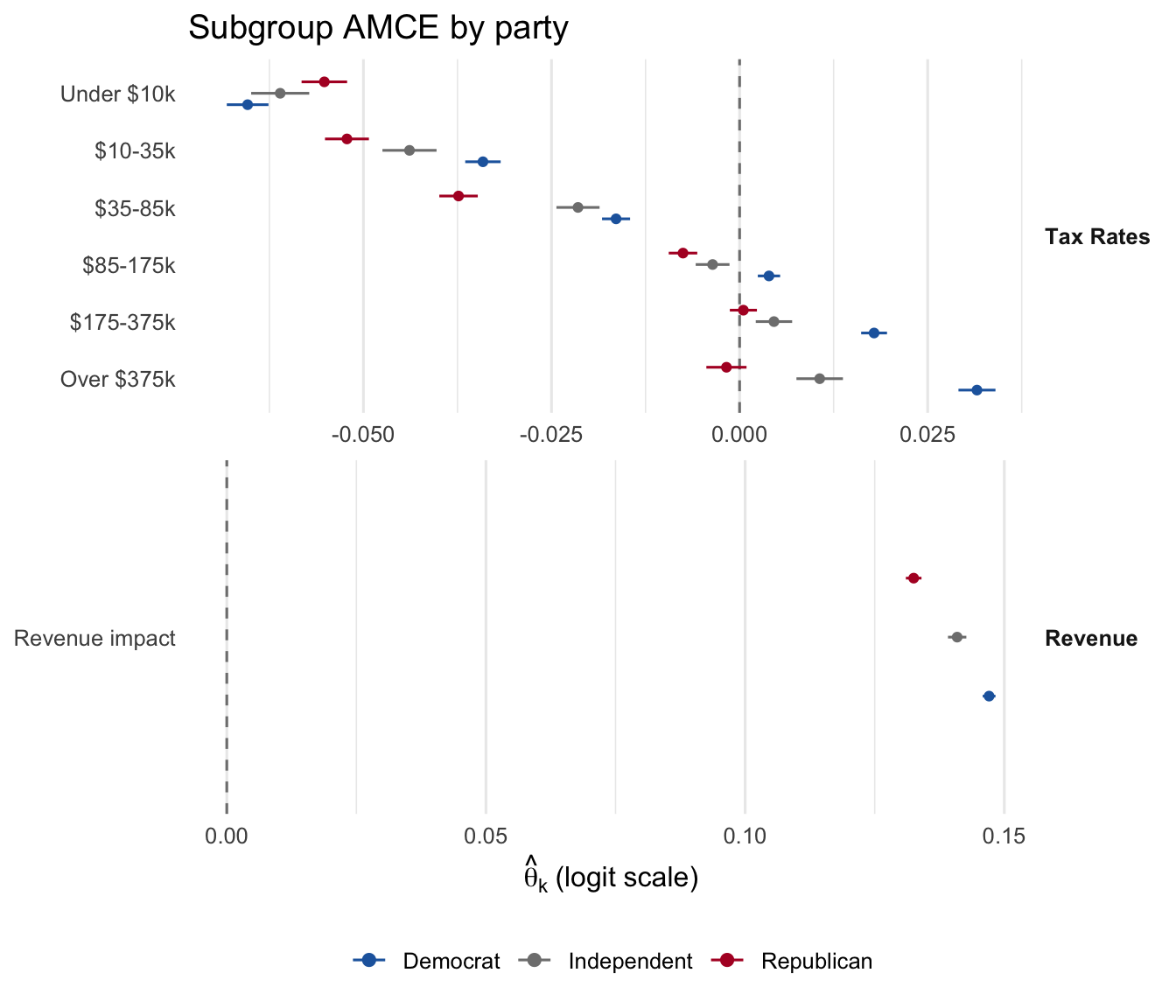
Party membership comes from the raw resp_pid7 convenience column (Democrat \(\le 3\), Independent \(= 4\), Republican \(\ge 5\)), mapped to the fit’s task rows. We reuse pid7_row from the importance chunk above.
plot_subgroup(
  fit_br,
  subgroup = list(
    Democrat    = pid7_row <= 3,
    Independent = pid7_row == 4,
    Republican  = pid7_row >= 5
  ),
  groups = br_groups, labels = br_labels,
  title = "Subgroup AMCE by party"
)
This plot is unique to the tax-plan conjoint. It extracts the six bracket coefficients \(\hat\beta_k(\mathbf Z_i)\) and shows the respondent-level preferred-rate schedule in three panels (one per party). The dark ribbon is the interquartile range across respondents within each party; the light ribbon is the 10th–90th percentile range.
## One row per respondent on the hybrid (MAP-refined) scale
beta_hat <- predict(fit_br, type = "beta")
first_row <- !duplicated(fit_br$respondent_id)
beta_resp <- beta_hat[first_row, ]

## Party assignment from the raw resp_pid7 convenience column
pid <- pid7_row[first_row]
party <- ifelse(pid <= 3, "Democrat",
         ifelse(pid >= 5, "Republican", "Independent"))

## Build schedule data: 6 brackets as x-axis, beta as y-axis
brackets <- c("Under $10k", "$10-35k", "$35-85k",
              "$85-175k", "$175-375k", "Over $375k")
rate_cols <- c("rate_L10", "rate_10_35", "rate_35_85",
               "rate_85_175", "rate_175_375", "rate_375P")

quant_data <- do.call(rbind, lapply(unique(party), function(p) {
  do.call(rbind, lapply(seq_along(brackets), function(j) {
    vals <- beta_resp[party == p, rate_cols[j]]
    data.frame(
      bracket = brackets[j],
      party   = p,
      median  = median(vals),
      q25     = quantile(vals, 0.25),
      q75     = quantile(vals, 0.75),
      q10     = quantile(vals, 0.10),
      q90     = quantile(vals, 0.90)
    )
  }))
}))
quant_data$bracket <- factor(quant_data$bracket, levels = brackets)
quant_data$party   <- factor(quant_data$party,
                              levels = c("Democrat", "Independent", "Republican"))

party_palette <- c(Democrat = "#2166AC", Independent = "gray50",
                   Republican = "#B2182B")

ggplot(quant_data, aes(x = bracket, color = party, fill = party, group = party)) +
  geom_ribbon(aes(ymin = q10, ymax = q90), alpha = 0.15, color = NA) +
  geom_ribbon(aes(ymin = q25, ymax = q75), alpha = 0.30, color = NA) +
  geom_line(aes(y = median), linewidth = 1.0) +
  geom_point(aes(y = median), size = 1.8) +
  geom_hline(yintercept = 0, linetype = "dashed", color = "gray50") +
  facet_wrap(~ party, ncol = 3) +
  scale_color_manual(values = party_palette, guide = "none") +
  scale_fill_manual(values  = party_palette, guide = "none") +
  labs(x = "Income bracket",
       y = expression(hat(beta)[k](Z) ~ "(utility per % point)"),
       title = "Tax schedule preferences, faceted by party") +
  theme_minimal(base_size = 11) +
  theme(axis.text.x = element_text(angle = 30, hjust = 1),
        strip.text  = element_text(face = "bold"))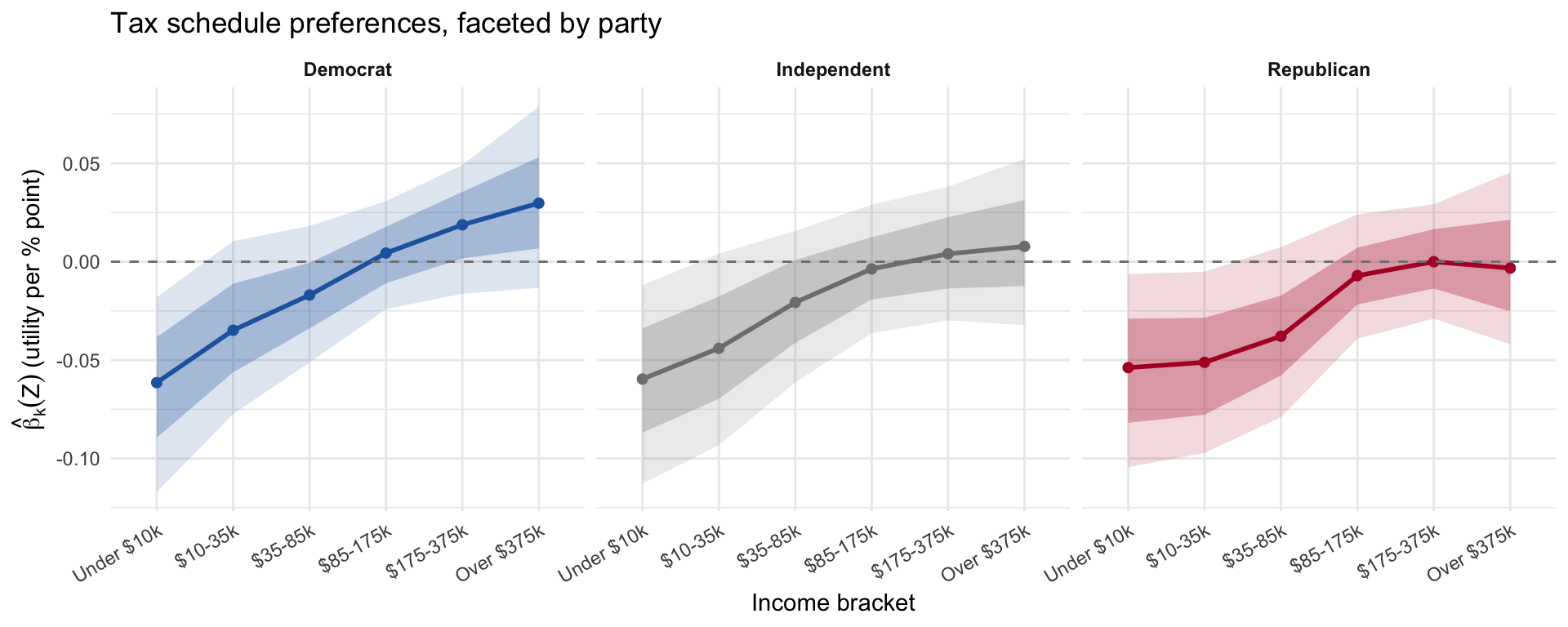
About 93% of respondents exhibit progressive tax preferences (a positive slope from low to high brackets), and 91% prefer a higher top-bracket rate than bottom-bracket rate. Progressivity remains the majority pattern even among Republicans (about 90% have a positive slope). The partisan gap is real but a matter of degree: the Democratic mean slope (about \(+0.021\)) is roughly 48% steeper than the Republican mean slope (about \(+0.014\)). Progressivity is the consensus; the parties differ on how steep, and — as the importance shares show — on which end of the schedule they care about most.
v_br <- sc_validate_amce(fit_br)
v_br
sc_validate_amce -- pooled and (optionally) subgroup comparison
Stage 2: varref
N obs: 16000, N respondents: 2000, P attributes: 7
Pooled correlation (DML theta vs homogeneous logit coef): 1
Pooled comparison (first 10 rows):
attribute dml_theta dml_se homog_logit_coef homog_logit_se diff
rate_L10 -0.06445 0.00372 -0.038785 0.000443 -0.02567
rate_10_35 -0.04360 0.00539 -0.026868 0.000655 -0.01673
rate_35_85 -0.02469 0.00295 -0.016207 0.000364 -0.00848
rate_85_175 -0.00295 0.00198 -0.000622 0.000265 -0.00232
rate_175_375 0.01002 0.00169 0.005481 0.000217 0.00454
rate_375P 0.01870 0.00202 0.010808 0.000240 0.00789
revenue_score 0.13959 0.04716 0.085723 0.006083 0.05386
abs_diff
0.02567
0.01673
0.00848
0.00232
0.00454
0.00789
0.05386Under correct logit specification, the DML \(\hat\theta\) on each tax bracket matches the pooled logit’s coefficient on the same bracket exactly. The pooled correlation is the cleanest summary that the structural model loses nothing the AMCE provides.
The tax application uses an all-continuous design:
As in the other applications, these schedule-level and subgroup quantities come from the individual preference vectors rather than from average marginal effects.