data(sw2022, package = "sconjoint")
dim(sw2022)
[1] 7146 37This chapter walks through a complete sconjoint analysis of the candidate-choice conjoint experiment of Saha and Weeks (2022). Respondents evaluate pairs of hypothetical political candidates and select one. The structural decomposition into direction and intensity lets us ask whether a near-zero average effect for candidate gender masks genuine heterogeneity — opposing camps of voters who prefer women and men.
The bundled sw2022 is the paper’s full analysis frame, so the quantities below reproduce the published estimates. The fit uses the paper’s production configuration (K = 10 cross-fitting folds and the default 1,000 Adam epochs); it is heavier than a quick demo and takes a couple of minutes to run.
Load the data and inspect its structure.
data(sw2022, package = "sconjoint")
dim(sw2022)[1] 7146 37The data are in long format: one row per respondent–task–profile. Each respondent contributes three forced-choice tasks; within a task two candidate profiles are presented and exactly one is chosen (choice == 1).
str(sw2022, list.len = 12)'data.frame': 7146 obs. of 37 variables:
$ respondent : chr "R_02LtLl5av6RqSoV" "R_02LtLl5av6RqSoV" "R_02LtLl5av6RqSoV" "R_02LtLl5av6RqSoV" ...
$ task : int 1 1 2 2 3 3 1 1 2 2 ...
$ profile : int 1 2 1 2 1 2 1 2 1 2 ...
$ choice : int 1 0 1 0 1 0 0 1 1 0 ...
$ cand_genderMale : num 1 0 0 0 1 1 0 1 1 0 ...
$ cand_runYes : num 1 1 0 0 1 0 1 0 1 1 ...
$ cand_talentCollaborative : num 0 0 0 0 0 0 0 1 0 0 ...
$ cand_talentDetermined.to.Succeed: num 0 0 0 0 0 1 0 0 0 0 ...
$ cand_talentEmpathetic : num 0 0 0 0 0 0 0 0 0 0 ...
$ cand_talentGood.Communicator : num 0 0 0 1 0 0 1 0 0 0 ...
$ cand_talentHard.Working : num 0 1 1 0 1 0 0 0 1 0 ...
$ cand_talentTough.Negotiator : num 1 0 0 0 0 0 0 0 0 0 ...
[list output truncated]table(table(sw2022$respondent))
   6
1191
The thirteen candidate attributes are already coded as 0/1 dummies, with the omitted level of each attribute serving as its reference (Female for gender, no prior run for ambition, and so on). The respondent-level moderators in \(\mathbf Z\) are the full set of nineteen covariates from the paper — gender, age, income, education, party, region, employment status, ideology, vote choice, and a gender-attitudes scale. The convenience factor resp_party (Democrat / Independent / Republican) is carried alongside for subgroup labelling but is not part of \(\mathbf Z\).
The formula interface puts conjoint attributes to the left of | and moderators to the right. Column names containing dots are backquoted:
attrs <- c("cand_genderMale", "cand_runYes",
           "cand_talentCollaborative", "cand_talentDetermined.to.Succeed",
           "cand_talentEmpathetic", "cand_talentGood.Communicator",
           "cand_talentHard.Working", "cand_talentTough.Negotiator",
           "cand_agendaModerate.Changes", "cand_agendaComplete.Overhaul",
           "cand_child1.child", "cand_child2.children", "cand_child3.children")
Zvars <- c("gender_num", "age", "income", "educ_Middle", "educ_High",
           "party_Republican", "party_Independent", "region_NORTHEAST",
           "region_SOUTH", "region_WEST", "employ_parttime",
           "employ_homemaker", "employ_not_working", "employ_retired",
           "employ_student", "ideo_conservative", "vote_trump",
           "vote_clinton", "gender_att")

bt  <- function(x) paste0("`", x, "`")
sw_formula <- stats::as.formula(
  paste("choice ~", paste(bt(attrs), collapse = " + "),
        "|",       paste(bt(Zvars), collapse = " + "))
)We fit the production configuration: K = 10 cross-fitting folds and the default 1,000 Adam epochs. This is the recipe that reproduces the paper, so the chunk is cached — rendering reuses the saved fit rather than retraining each time. The loss trace later in the chapter shows the per-fold training curves.
fit_sw <- scfit(
  sw_formula,
  data       = sw2022,
  respondent = "respondent",
  task       = "task",
  profile    = "profile",
  K          = 10L,
  seed       = 42L,
  stage2     = "map_c5",
  parallel   = TRUE,
  n_cores    = 10L
)
summary(fit_sw)
sc_fit summary
Call: scfit(formula = sw_formula, data = sw2022, respondent = "respondent",
task = "task", profile = "profile", K = 10L, seed = 42L,
parallel = TRUE, n_cores = 10L, stage2 = "map_c5")
1191 respondents | 3573 observations | K = 10 folds
hidden = 32-32-16 | epochs = 1000 | seed = 42 | device = cpu | parallel (10 cores)
Coefficients (DML, respondent-clustered SE):
estimate std_error z_value p_value
cand_genderMale -0.10309 0.06847 -1.5055 1.322e-01
cand_runYes 0.05932 0.06830 0.8684 3.851e-01
cand_talentCollaborative 0.18081 0.11827 1.5288 1.263e-01
cand_talentDetermined.to.Succeed 0.26879 0.11525 2.3323 1.969e-02
cand_talentEmpathetic 0.06556 0.12456 0.5263 5.987e-01
cand_talentGood.Communicator 0.25585 0.11803 2.1676 3.019e-02
cand_talentHard.Working 0.54652 0.11942 4.5763 4.732e-06
cand_talentTough.Negotiator 0.16607 0.11643 1.4264 1.538e-01
cand_agendaModerate.Changes 0.95279 0.08493 11.2189 3.293e-29
cand_agendaComplete.Overhaul 0.94238 0.09733 9.6820 3.597e-22
cand_child1.child 0.26575 0.09388 2.8308 4.643e-03
cand_child2.children 0.42296 0.09278 4.5588 5.146e-06
cand_child3.children 0.51191 0.09074 5.6416 1.685e-08
ci_lo ci_hi
cand_genderMale -0.23729 0.03112
cand_runYes -0.07456 0.19319
cand_talentCollaborative -0.05099 0.41261
cand_talentDetermined.to.Succeed 0.04291 0.49467
cand_talentEmpathetic -0.17857 0.30969
cand_talentGood.Communicator 0.02451 0.48719
cand_talentHard.Working 0.31246 0.78059
cand_talentTough.Negotiator -0.06212 0.39427
cand_agendaModerate.Changes 0.78634 1.11925
cand_agendaComplete.Overhaul 0.75161 1.13315
cand_child1.child 0.08175 0.44974
cand_child2.children 0.24112 0.60481
cand_child3.children 0.33407 0.68976
DML/iid SE ratio (mean): 1.032
Stage 2: map_c5 | mean(sigma_prior) = 0.1272scfit() reports Stage 2: map_c5, the empirical-Bayes MAP refinement that runs by default; Chapter 3 explains the Stage-1 / Stage-2 split and the stage2 options. DML estimates use the Stage-1 DNN (fit_sw$beta_hat_dnn); the refined fit_sw$beta_hat feeds the distributional and individual-level quantities below.
The DML point estimates \(\hat\theta_k\) on the logit scale. Inspect numerically, then visualize as a coefficient plot grouped by attribute.
coef(fit_sw) cand_genderMale cand_runYes
-0.10308858 0.05931866
cand_talentCollaborative cand_talentDetermined.to.Succeed
0.18081164 0.26878850
cand_talentEmpathetic cand_talentGood.Communicator
0.06555814 0.25584984
cand_talentHard.Working cand_talentTough.Negotiator
0.54652422 0.16607249
cand_agendaModerate.Changes cand_agendaComplete.Overhaul
0.95279401 0.94237735
cand_child1.child cand_child2.children
0.26574584 0.42296203
cand_child3.children
0.51191480 Agenda dominates: relative to keeping the status quo, both moderate changes and a complete overhaul raise candidate utility by about 0.95 on the logit scale. Among the talent cues, hard-working is the strongest (about +0.55). The average effect of a male candidate is small and negative (about \(-0.10\), confidence interval covering zero) — the near-zero average we return to below.
plot_amce(fit_sw, groups = sw_groups, labels = sw_labels)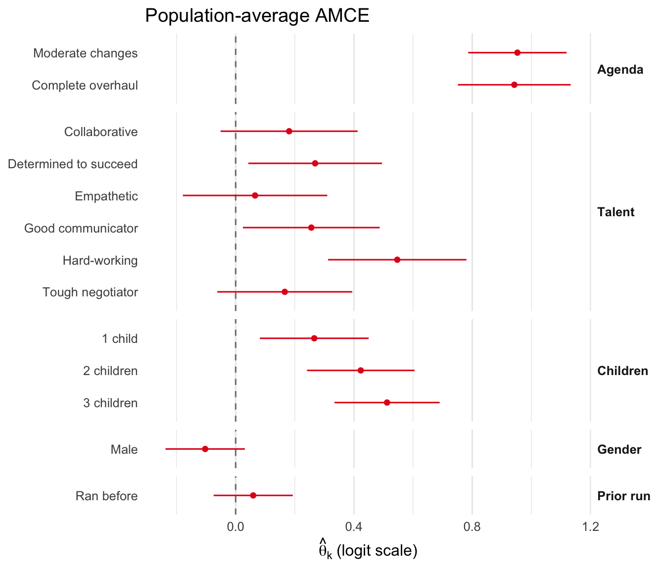
The structural model’s average marginal effect (AME) on the probability scale nearly coincides with the standard linear-probability-model AMCE, confirming that the structural estimator nests reduced-form AMCE analysis. We compute both and overlay them as point-ranges on the probability scale.
## Structural AME on the probability scale (delta-method via plogis')
ame_struct <- sc_average(fit_sw, scale = "probability")
ame_df     <- ame_struct$estimate
ame_df$source <- "Structural AME"

## Linear-probability-model AMCE
lpm        <- sc_baseline_lpm(fit_sw)
amce_df    <- data.frame(
  dummy_name = names(stats::coef(lpm)),
  estimate   = unname(stats::coef(lpm)),
  se         = sqrt(diag(stats::vcov(lpm))),
  source     = "LPM AMCE",
  stringsAsFactors = FALSE
)
amce_df$ci_lo <- amce_df$estimate - 1.96 * amce_df$se
amce_df$ci_hi <- amce_df$estimate + 1.96 * amce_df$se

df_both <- rbind(
  ame_df[, c("dummy_name", "estimate", "se", "ci_lo", "ci_hi", "source")],
  amce_df[amce_df$dummy_name %in% names(sw_labels),
          c("dummy_name", "estimate", "se", "ci_lo", "ci_hi", "source")]
)
df_both$label <- sw_labels[df_both$dummy_name]
df_both$label <- factor(df_both$label, levels = rev(unname(sw_labels)))
df_both$group <- sw_groups[df_both$dummy_name]
df_both$group <- factor(df_both$group, levels = unique(sw_groups))

ggplot(df_both, aes(x = estimate, y = label, color = source)) +
  geom_vline(xintercept = 0, linetype = "dashed", color = "gray50") +
  geom_pointrange(aes(xmin = ci_lo, xmax = ci_hi),
                  position = position_dodge(width = 0.5),
                  size = 0.35, fatten = 2) +
  scale_color_manual(values = c("Structural AME" = "#2166AC",
                                "LPM AMCE"        = "#B2182B")) +
  facet_grid(group ~ ., scales = "free_y", space = "free_y") +
  labs(x = "Effect on Pr(choice)",
       y = NULL, color = NULL,
       title = "Structural AME vs LPM AMCE (probability scale)") +
  theme_minimal(base_size = 11) +
  theme(legend.position = "bottom",
        strip.text.y    = element_text(angle = 0, hjust = 0, face = "bold"))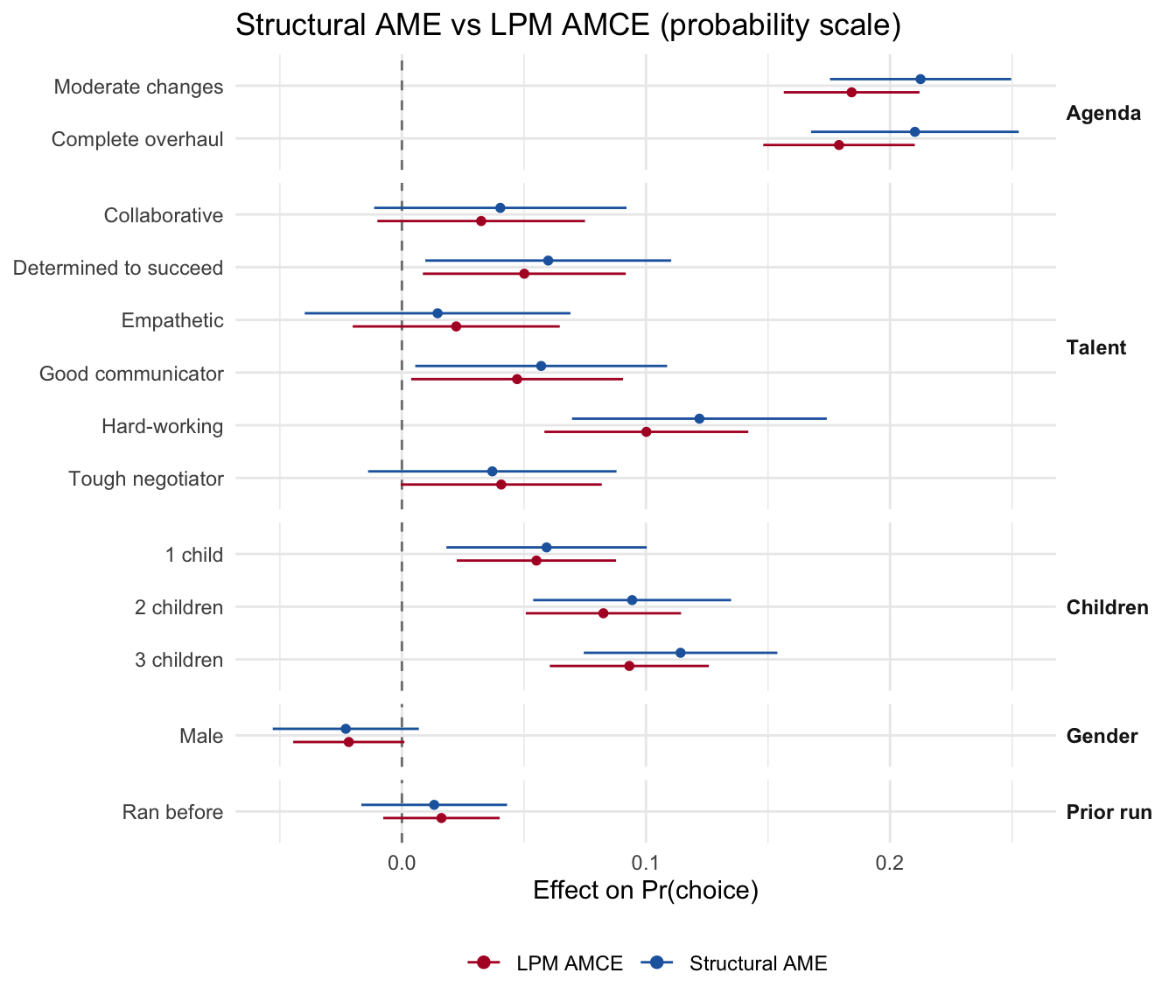
The two series overlap nearly point-for-point: the structural model loses nothing the reduced-form AMCE provides. The sc_validate_amce() check at the end of the chapter quantifies this agreement.
Pull the respondent-level \(\hat\beta(\mathbf Z_i)\) matrix. With the default stage2 = "map_c5", this is the MAP-refined hybrid view.
beta <- predict(fit_sw)
dim(beta)
[1] 3573 13round(beta[1:3, 1:6], 2) cand_genderMale cand_runYes cand_talentCollaborative
[1,] -0.08 0.25 0.19
[2,] -0.08 0.25 0.19
[3,] -0.08 0.25 0.19
cand_talentDetermined.to.Succeed cand_talentEmpathetic
[1,] 0.26 0.21
[2,] 0.26 0.21
[3,] 0.26 0.21
cand_talentGood.Communicator
[1,] 0.29
[2,] 0.29
[3,] 0.29Ridgeline densities show the distribution of \(\hat\beta_k(\mathbf Z_i)\) per dummy across respondents. The vertical dashed line is at zero; the solid line in each density is the median.
plot(fit_sw, "beta_ridgelines", groups = sw_groups, labels = sw_labels)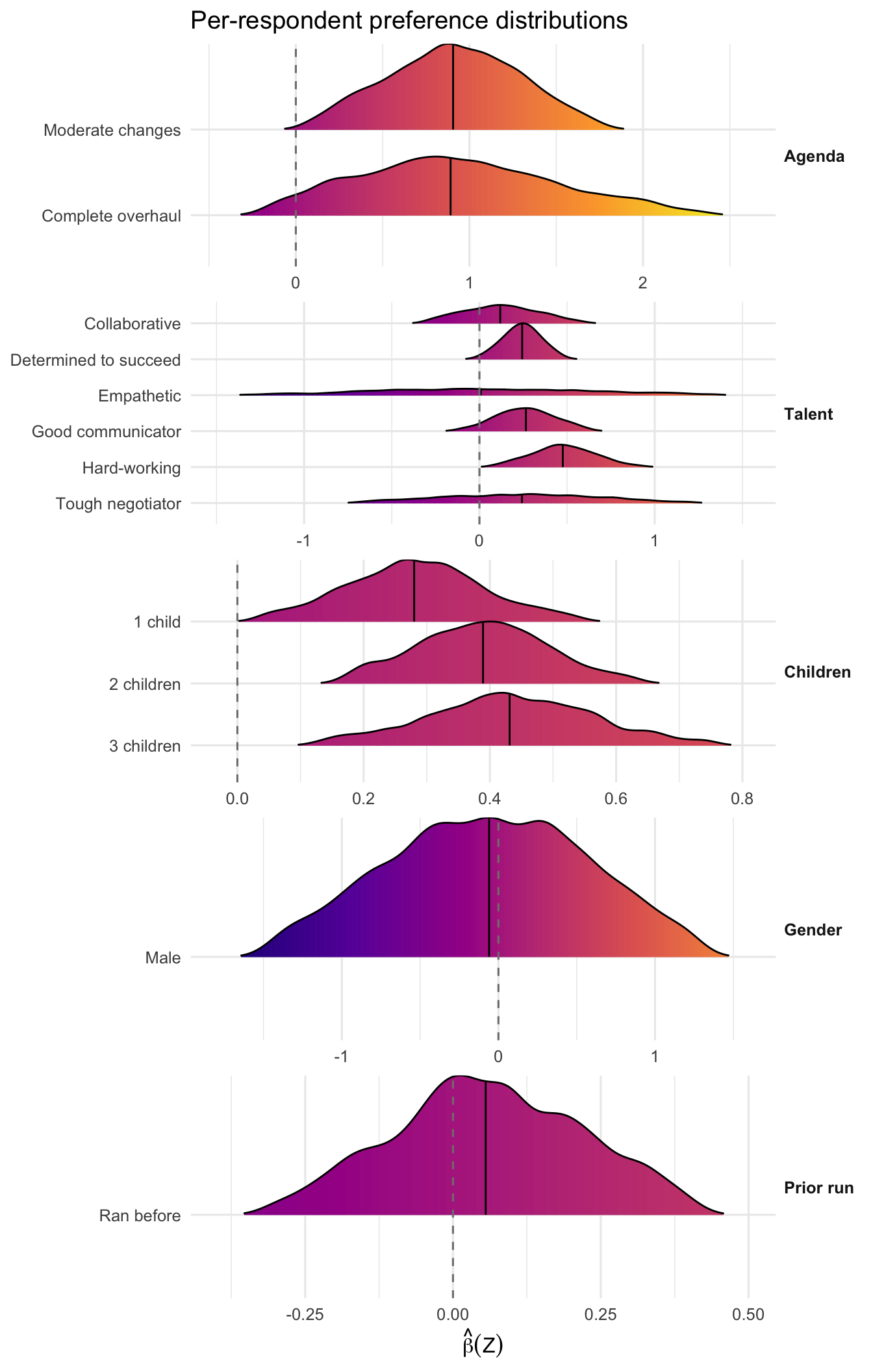
The gender density is centred just left of zero but spreads to both sides — the visual signature of two opposing camps rather than a shared near-indifference, a pattern we make precise next.
The variance-decomposition share of utility carried by each attribute, averaged across respondents. Importance answers: which attribute moves the choice the most? Because the bundled formula enters each level as a separate dummy, we first tell sc_importance() which dummies belong to the same attribute (via the sw_attr_map() helper defined in the setup chunk), then read off the paper’s five-attribute decomposition.
fit_grp <- sw_attr_map(fit_sw)
imp <- sc_importance(fit_grp, design = "uniform")
imp$estimate[, c("attribute", "share", "se")]
attribute share se
1 cand_gender 0.16051704 0.0037788949
2 cand_run 0.02033821 0.0009475866
3 cand_talent 0.20272507 0.0031909265
4 cand_agenda 0.53135141 0.0054917708
5 cand_child 0.08506827 0.0015072658plot_importance(fit_grp, labels = c(
cand_agenda = "Agenda", cand_talent = "Talent",
cand_child = "Children", cand_gender = "Gender", cand_run = "Prior run"))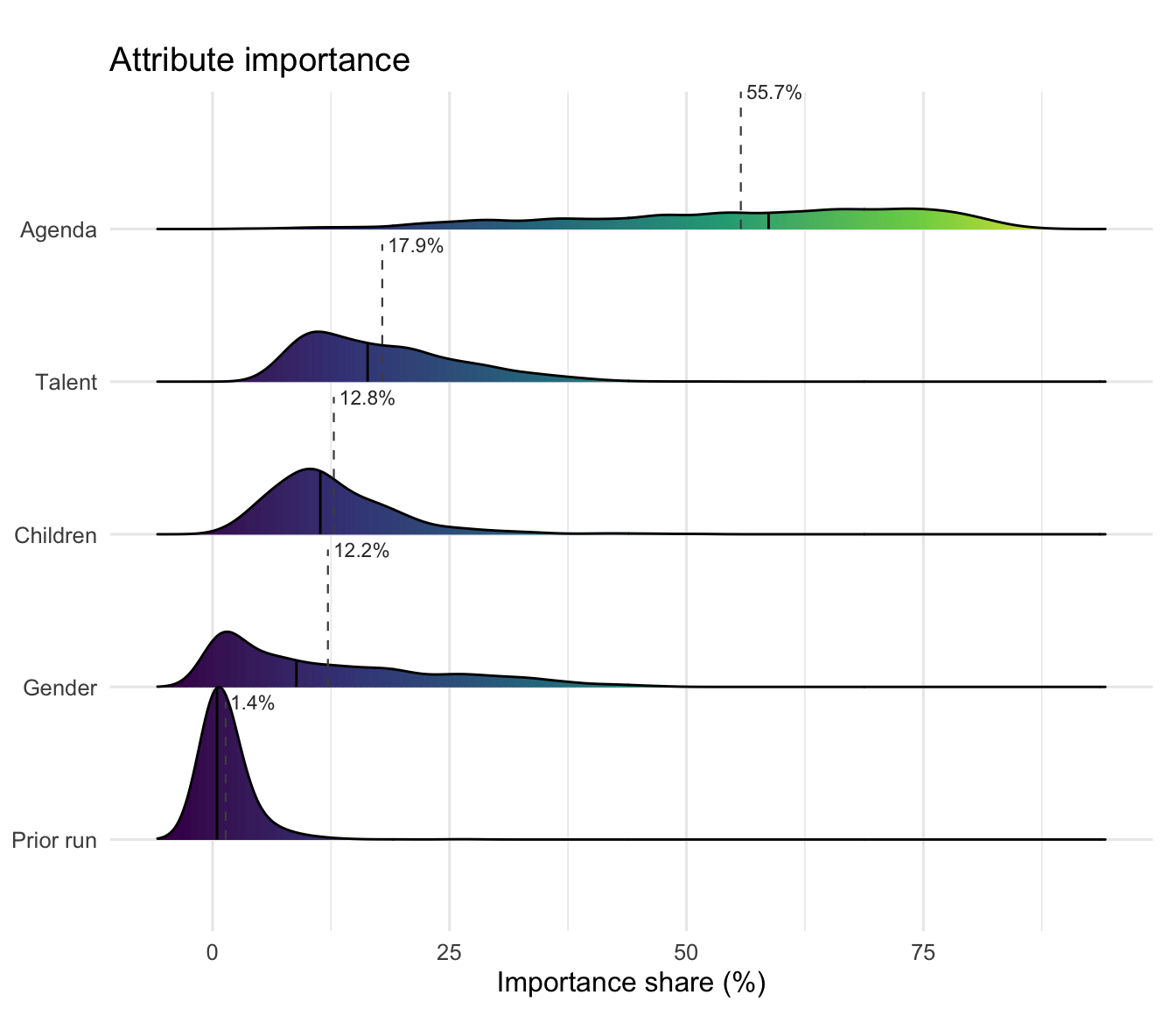
Policy agenda dominates the decision variance, carrying roughly half the explained variation. Candidate gender accounts for about 16% of the variance — the third-largest attribute, behind agenda and talent and well ahead of children and prior office. This is the first sign that gender matters far more than its near-zero average effect suggests: the variance is large precisely because respondents disagree about its sign.
For each dummy, decompose preference into a direction (the sign of \(\hat\beta_{ik}\)) and an intensity (its magnitude). A near-zero average effect can hide either consensus (everyone close to zero) or polarization (large opposing intensities cancelling).
sc_direction_intensity(fit_sw)sc_quantity_bivariate: direction_intensity
-- direction --
sc_quantity: direction
estimate: data.frame with 13 rows
dummy_name d se_d ci_lo_d ci_hi_d
cand_genderMale -0.06969 0.028918 -0.1264 -0.01301
cand_runYes 0.25945 0.027996 0.2046 0.31432
cand_talentCollaborative 0.38203 0.026790 0.3295 0.43454
cand_talentDetermined.to.Succeed 0.94962 0.009085 0.9318 0.96743
cand_talentEmpathetic 0.01092 0.028987 -0.0459 0.06773
cand_talentGood.Communicator 0.84215 0.015632 0.8115 0.87279
cand_talentHard.Working 0.97649 0.006249 0.9642 0.98874
cand_talentTough.Negotiator 0.35013 0.027154 0.2969 0.40335
cand_agendaModerate.Changes 0.97817 0.006024 0.9664 0.98998
cand_agendaComplete.Overhaul 0.88077 0.013727 0.8539 0.90768
... 3 more rows
-- intensity --
sc_quantity: intensity
estimate: data.frame with 13 rows
dummy_name u se_u ci_lo_u ci_hi_u
cand_genderMale 0.5744 0.012386 0.5502 0.5987
cand_runYes 0.1523 0.003455 0.1455 0.1590
cand_talentCollaborative 0.2136 0.004637 0.2045 0.2227
cand_talentDetermined.to.Succeed 0.2449 0.003271 0.2385 0.2513
cand_talentEmpathetic 0.5609 0.012312 0.5368 0.5850
cand_talentGood.Communicator 0.2769 0.004781 0.2675 0.2862
cand_talentHard.Working 0.4838 0.006025 0.4720 0.4956
cand_talentTough.Negotiator 0.4464 0.009701 0.4274 0.4655
cand_agendaModerate.Changes 0.9121 0.012158 0.8882 0.9359
cand_agendaComplete.Overhaul 0.9713 0.017771 0.9364 1.0061
... 3 more rowsCandidate gender is the paper’s clearest example of cancellation: its direction summary sits near zero (a slim majority lean toward female candidates), but its intensity is substantial — the opposing camps hold their preferences with real strength, and they cancel in the average.
What share of respondents have a positive coefficient on each dummy? This is the direction-only summary — it ignores intensity.
frac <- sc_fraction_preferring(fit_sw, threshold = 0)
frac$estimate[, c("dummy_name", "frac_positive", "frac_negative")]
dummy_name frac_positive frac_negative
1 cand_genderMale 0.4651553 0.534844668
2 cand_runYes 0.6297229 0.370277078
3 cand_talentCollaborative 0.6910160 0.308984047
4 cand_talentDetermined.to.Succeed 0.9748111 0.025188917
5 cand_talentEmpathetic 0.5054576 0.494542401
6 cand_talentGood.Communicator 0.9210747 0.078925273
7 cand_talentHard.Working 0.9882452 0.011754828
8 cand_talentTough.Negotiator 0.6750630 0.324937028
9 cand_agendaModerate.Changes 0.9890848 0.010915197
10 cand_agendaComplete.Overhaul 0.9403862 0.059613770
11 cand_child1.child 0.9840470 0.015952981
12 cand_child2.children 1.0000000 0.000000000
13 cand_child3.children 0.9949622 0.005037783plot_fraction(fit_sw, groups = sw_groups, labels = sw_labels)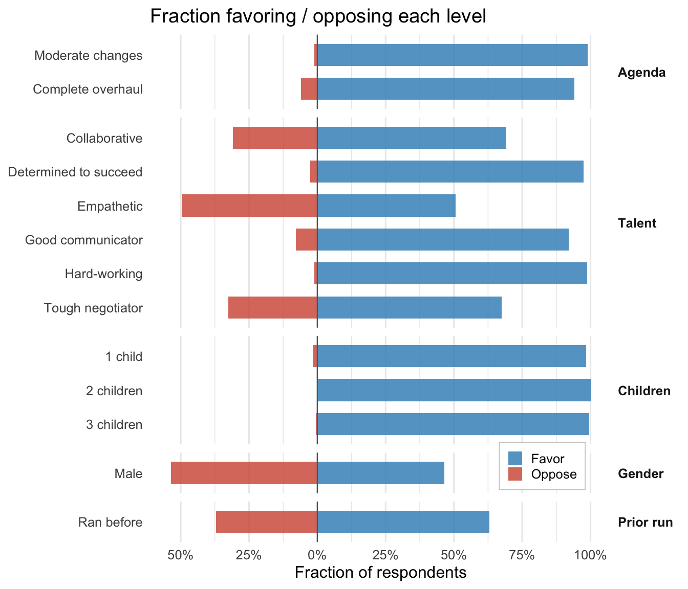
The directional finding for gender: the population-average effect for male is near zero, yet a clear majority of respondents have \(\hat\beta_{\text{Male}} < 0\) — about 54% prefer female candidates against 46% who prefer men. The electorate is split close to evenly on gender, not indifferent to it. The partisan structure behind that split appears in the subgroup section below.
The respondent-averaged trimmed ratio \(\hat\beta_j / \hat\beta_k\) between two dummies, with respondent-clustered SE. Trimming at \(\{0.01, 0.99\}\) guards the unbounded ratio when the denominator is near zero.
sc_mrs(fit_sw, numerator = 1L, denominator = 2L)sc_quantity: mrs
estimate = -1.679 se = 0.812 95% CI = [-3.271, -0.08798]The ratio \(\hat\beta_j / \hat\beta_k\) is unbounded when the denominator is near zero. Here the numerator is the male dummy, whose recovered effect is near zero for many respondents, so the ratio is noisy; inspect the ridgelines above to confirm the denominator column is well-separated from zero before reading a MRS literally.
Predicted choice probability for a specific head-to-head profile pair, averaged across respondents. Each profile is a named list of dummy settings; unmentioned dummies stay at zero (the reference level).
sc_counterfactual(
  fit_sw,
  ## Profile A: a Female, Empathetic candidate proposing a Complete
  ## Overhaul, with two children and a prior run for office. Female is
  ## the reference level, so cand_genderMale stays 0.
  ## Profile B: a Male, Tough-Negotiator candidate with no prior run and
  ## the omitted (status-quo) agenda.
  A = list(cand_talentEmpathetic = 1, cand_agendaComplete.Overhaul = 1,
           cand_child2.children = 1, cand_runYes = 1),
  B = list(cand_genderMale = 1, cand_talentTough.Negotiator = 1)
)
sc_quantity: counterfactual
estimate = 0.7631 se = 0.03403 95% CI = [0.6964, 0.8298]The single profile that maximizes the population-average utility (greedy attribute-by-attribute selection over the discrete attribute levels).
sc_optimal_profile(fit_sw)sc_quantity: optimal_profile
estimate = 0.9773 se = 0.0008319 95% CI = [0.9757, 0.9789]For each dummy, the one-sided test that \(\mathrm{Var}(\beta_k(Z)) > 0\). Useful for screening which attributes genuinely vary across respondents.
sc_heterogeneity_test(fit_sw, adjust = "bh")sc_quantity: heterogeneity_test
estimate: data.frame with 13 rows
dummy_name var_beta se_var t_stat p_value
cand_genderMale 0.50773 0.0203844 24.91 3.053e-137
cand_runYes 0.03394 0.0014738 23.03 1.266e-117
cand_talentCollaborative 0.05622 0.0023005 24.44 3.560e-132
cand_talentDetermined.to.Succeed 0.01427 0.0006844 20.85 6.901e-97
cand_talentEmpathetic 0.49426 0.0205142 24.09 1.462e-128
cand_talentGood.Communicator 0.03531 0.0015258 23.14 8.429e-119
cand_talentHard.Working 0.04462 0.0021305 20.95 1.041e-97
cand_talentTough.Negotiator 0.25649 0.0109576 23.41 1.800e-121
cand_agendaModerate.Changes 0.17947 0.0071617 25.06 6.757e-139
cand_agendaComplete.Overhaul 0.43795 0.0206981 21.16 1.145e-99
p_adjusted sig
1.984e-136 ***
2.352e-117 ***
1.543e-131 ***
8.155e-97 ***
4.753e-128 ***
1.826e-118 ***
1.353e-97 ***
4.680e-121 ***
8.784e-138 ***
1.654e-99 ***
... 3 more rowsplot_hetero(fit_sw, groups = sw_groups, labels = sw_labels)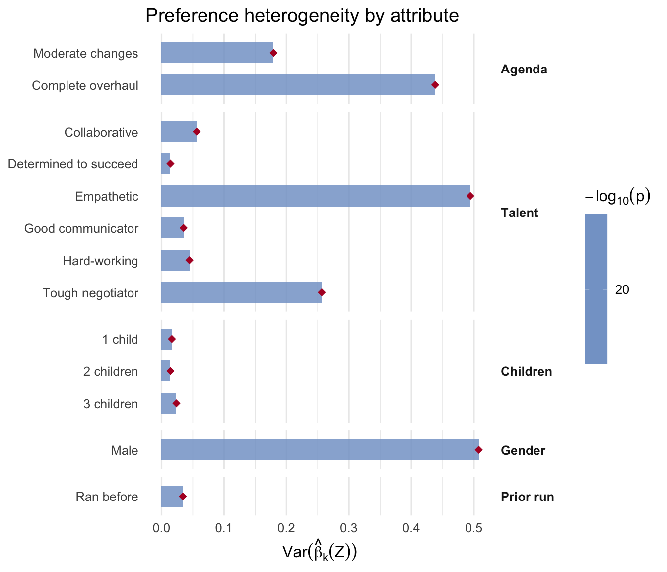
Candidate gender shows highly significant variance in \(\beta(Z)\) — the formal counterpart to this cancellation: the spread around the near-zero mean is real, not sampling noise.
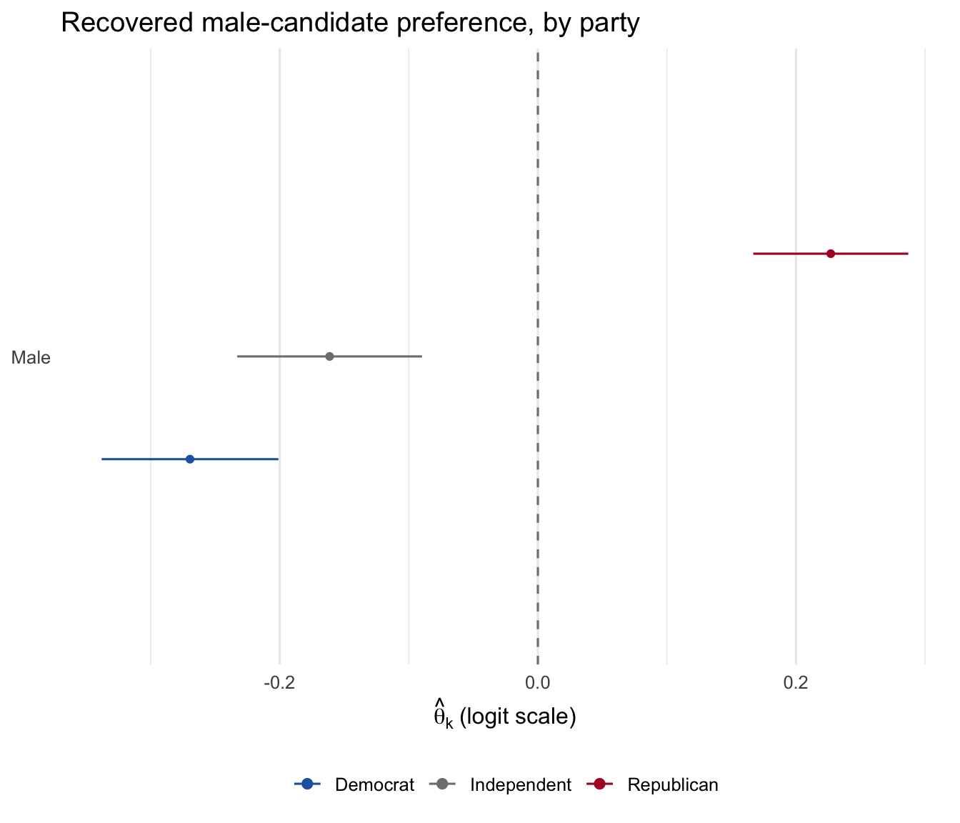
Re-average the respondent-level betas over a subset of respondents, then compare across subsets. The paper’s main result is partisan: the null average effect of gender masks Democrats who prefer women and Republicans who prefer men. We recover it by splitting on resp_party. Subgroup masks are aligned to the rows of fit_sw$beta_hat, which Z shares, so we build them from the party indicators in fit_sw$Z.
Z   <- fit_sw$Z
dem <- Z[, "party_Republican"] == 0 & Z[, "party_Independent"] == 0
ind <- Z[, "party_Independent"] == 1
rep <- Z[, "party_Republican"] == 1

male_row <- function(mask) {
  s <- sc_subgroup(fit_sw, mask)
  s$estimate[s$estimate$dummy_name == "cand_genderMale", c("theta", "se")]
}
rbind(
  Democrat    = male_row(dem),
  Independent = male_row(ind),
  Republican  = male_row(rep)
)
theta se
Democrat -0.2695236 0.03494222
Independent -0.1613402 0.03652892
Republican 0.2269224 0.03063728The recovered party means show the paper’s finding directly: the average male coefficient is clearly negative for Democrats (they prefer women), clearly positive for Republicans (they prefer men), and near zero for Independents. Two camps of comparable strength pull in opposite directions, and the overall average lands near zero by cancellation, not by indifference.
plot_subgroup(
  fit_sw,
  subgroup = list(Democrat = dem, Independent = ind, Republican = rep),
  dummies  = "cand_genderMale",
  labels   = sw_labels,
  title    = "Recovered male-candidate preference, by party"
)
We can run the same split on the respondent’s own gender, coded in the standardized moderator gender_num (its two levels label the two coded groups; the package does not store which sign is female, so we keep the labels neutral):
g_lo <- fit_sw$Z[, "gender_num"] < 0
g_hi <- fit_sw$Z[, "gender_num"] > 0
rbind(
  `gender_num < 0` = male_row(g_lo),
  `gender_num > 0` = male_row(g_hi)
)
theta se
gender_num < 0 -0.19362972 0.02864491
gender_num > 0 0.05204795 0.02891781plot(fit_sw, "loss_trace")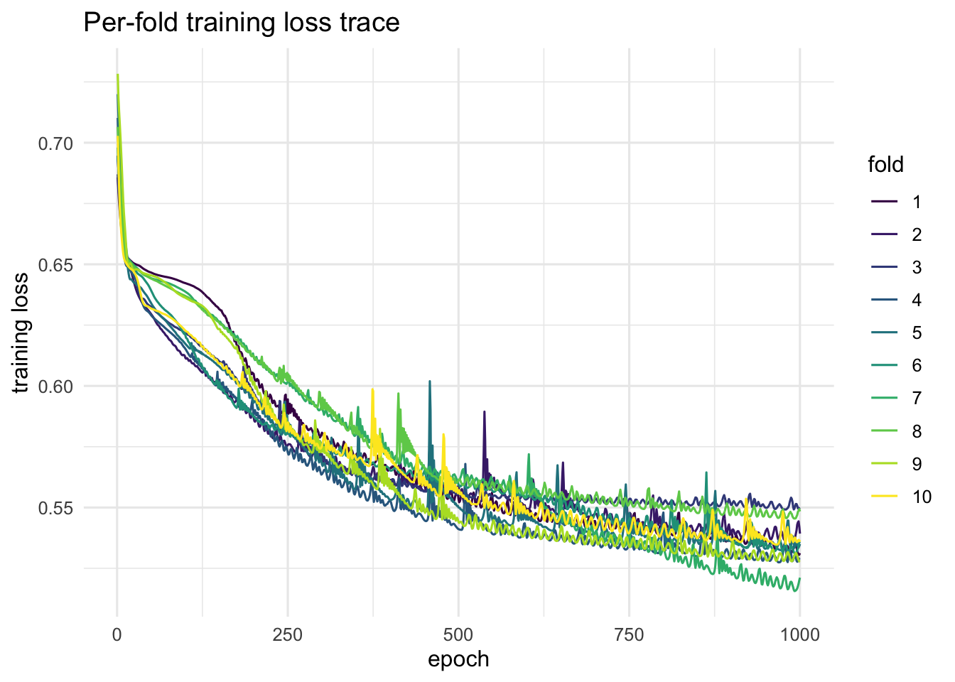
sc_design_diagnostic() estimates per-coefficient \(\hat R^2_{Z,k}\) from the MAP posterior and reports which recovery tiers the design supports (mean / distributional / individual / ratio) per the paper’s design-guidance heuristics. On the Saha-Weeks design (three tasks per respondent, the full nineteen-covariate set) the talent attributes are well pinned by \(\mathbf Z\), while gender, prior run, and children rely most on the within-respondent task variation.
sc_design_diagnostic(fit_sw)sc_design_diagnostic --- recovery-tier hint
[experimental: estimator over-estimates R^2_Z when Z is
uninformative (validation bias +0.4 at true R^2_Z = 0.10).
Use for relative comparisons across coefficients; do not
treat tier hints as a pass/fail gate. See ?sc_design_diagnostic.]
Stage 2: map_c5
Respondents: 1191 | Tasks: 3573 | T_mean: 3 | mean R^2_Z: 0.594
Recovery tiers:
[YES] mean & aggregate (any reasonable design)
[NO] distributional (T >= 5 and R^2_Z >= 0.35)
[NO] individual-level (T >= 8 and R^2_Z >= 0.55)
[NO] ratio (MRS / WTP) (T >= 10 and R^2_Z >= 0.55 and N >= 5000)
Top coefficients by R^2_Z (best-pinned by Z):
cand_talentTough.Negotiator 0.992
cand_talentCollaborative 0.966
cand_talentHard.Working 0.957
cand_talentEmpathetic 0.951
cand_talentGood.Communicator 0.946
Bottom coefficients (rely most on T for recovery):
cand_agendaModerate.Changes 0.429
cand_child3.children 0.157
cand_child1.child 0.0895
cand_runYes 0.0612
cand_child2.children 0.06The paper’s Supplementary Materials (Section D) show that the structural model nests the standard reduced-form AMCE: the DML population-average parameter \(\theta_k = \mathbb{E}[\beta_k(Z)]\) equals the pooled homogeneous-logit coefficient on attribute \(k\) when the logit specification holds. The sc_validate_amce() export turns this into a one-line sanity check.
v <- sc_validate_amce(fit_sw)
v
sc_validate_amce -- pooled and (optionally) subgroup comparison
Stage 2: map_c5
N obs: 3573, N respondents: 1191, P attributes: 13
Pooled correlation (DML theta vs homogeneous logit coef): 0.997
Pooled comparison (first 10 rows):
attribute dml_theta dml_se homog_logit_coef
cand_genderMale -0.1031 0.0685 -0.0952
cand_runYes 0.0593 0.0683 0.0699
cand_talentCollaborative 0.1808 0.1183 0.1393
cand_talentDetermined.to.Succeed 0.2688 0.1152 0.2163
cand_talentEmpathetic 0.0656 0.1246 0.0959
cand_talentGood.Communicator 0.2558 0.1180 0.2040
cand_talentHard.Working 0.5465 0.1194 0.4352
cand_talentTough.Negotiator 0.1661 0.1164 0.1757
cand_agendaModerate.Changes 0.9528 0.0849 0.7914
cand_agendaComplete.Overhaul 0.9424 0.0973 0.7696
homog_logit_se diff abs_diff
0.0116 -0.00791 0.00791
0.0122 -0.01061 0.01061
0.0217 0.04149 0.04149
0.0212 0.05248 0.05248
0.0216 -0.03033 0.03033
0.0221 0.05186 0.05186
0.0213 0.11132 0.11132
0.0210 -0.00967 0.00967
0.0142 0.16143 0.16143
0.0158 0.17282 0.17282At the production configuration used here (K = 10, 1,000 epochs) the correlation across attribute levels is very high (close to 1), confirming that the structural estimator reproduces the reduced-form benchmark. A material drop would signal either insufficient training or a genuinely non-logit data-generating process.
Every sc_* quantity accepts a which_beta argument with default "hybrid" (Stage-2 refined). Passing "dnn" reads the unrefined Stage-1 DNN mean, which lives in fit_sw$beta_hat_dnn.
frac_hyb <- sc_fraction_preferring(fit_sw, which_beta = "hybrid")
frac_dnn <- sc_fraction_preferring(fit_sw, which_beta = "dnn")
data.frame(
  attribute   = frac_hyb$estimate$dummy_name,
  hybrid_pref = round(frac_hyb$estimate$frac_positive, 3),
  dnn_pref    = round(frac_dnn$estimate$frac_positive, 3)
)
attribute hybrid_pref dnn_pref
1 cand_genderMale 0.465 0.433
2 cand_runYes 0.630 0.736
3 cand_talentCollaborative 0.691 0.720
4 cand_talentDetermined.to.Succeed 0.975 0.931
5 cand_talentEmpathetic 0.505 0.541
6 cand_talentGood.Communicator 0.921 0.919
7 cand_talentHard.Working 0.988 0.970
8 cand_talentTough.Negotiator 0.675 0.668
9 cand_agendaModerate.Changes 0.989 0.983
10 cand_agendaComplete.Overhaul 0.940 0.893
11 cand_child1.child 0.984 0.963
12 cand_child2.children 1.000 0.994
13 cand_child3.children 0.995 0.990The hybrid and raw-DNN fractions can differ because the Stage-2 MAP update pulls each respondent’s coefficients toward the mean stage. How much a column’s fraction moves — and in which direction — depends on how much it leaned on noisy individual variation; compare the two columns in the table above.
The candidate application is the clearest illustration of why averages can mislead: