3  Example: Democratic Norms

This chapter applies the structural estimator to a candidate-choice conjoint whose design follows Graham and Svolik (2020). Respondents choose between pairs of hypothetical U.S. candidates; one attribute captures the candidate’s willingness to engage in undemocratic behavior (ignoring a court ruling, restricting the opposition press, or banning an opposition rally). The original study asks how much voters penalize co-partisan candidates for violating democratic norms, and whether strong partisanship leads to tolerance of such violations.

The structural model adds value here because it decomposes the population-average penalty for undemocratic behavior into direction and intensity, and traces the heterogeneity back to respondent-level partisanship — without re-estimating on subsets.

The bundled gs2020 data is the paper’s full analysis frame, and this chapter reproduces the paper’s main (held-out) specification: the 16-covariate moderator set that drops the six direct democracy-attitude items (see Fitting the structural model, below). The numbers reported here match the paper’s Section 4.2.

3.1 Data preparation

Load the Graham-Svolik analysis frame and inspect its structure. Each respondent contributes about 13 forced-choice tasks against pairs of hypothetical candidates.

data(gs2020, package = "sconjoint")
dim(gs2020)
[1] 41314    59
gs2020[1:4, c("respondent", "task", "profile", "choice",
              "diff_respParty", "diff_dem_code_u_journalists")]
  respondent task profile choice diff_respParty diff_dem_code_u_journalists
1     000001    1       1      0              0                           0
2     000001    1       2      1              0                           0
3     000001    2       1      1              0                           0
4     000001    2       2      0              0                           0

Every sconjoint input is in long format: one row per respondent–task–profile, with exactly one profile chosen in each task (choice == 1). This frame follows that convention, and it is already in the paper’s two-profile parameterization: the choice outcome, the identifiers (respondent, task, profile), 30 attribute contrasts (the diff_ columns, differenced across the two profiles), and the respondent-level moderators \(\mathbf{Z}\) (the z_* and *_ideal columns plus six direct democracy-attitude items). Because the design is differenced, the reference levels are already absorbed (good governance is measured against an “elect oversight board” baseline; the undemocratic and valence items against “absent” and “no scandal”). No re-leveling is needed.

The 15 undemocratic, good-governance, and valence contrasts split into three families: good-governance (diff_dem_code_g_*, 6 contrasts), undemocratic actions (diff_dem_code_u_*, 7 contrasts), and valence violations (diff_dem_code_v_*, 2 contrasts). Their raw conditional choice rates make the families clear: candidates who endorse an undemocratic action or carry a valence scandal are chosen far less often.

u_cols <- grep("^diff_dem_code_u_", names(gs2020), value = TRUE)
v_cols <- grep("^diff_dem_code_v_", names(gs2020), value = TRUE)
## Mean choice rate for the profile carrying each contrast (diff == 1)
rate_when_present <- function(col) {
  mean(gs2020$choice[gs2020[[col]] == 1])
}
round(sort(sapply(c(u_cols, v_cols), rate_when_present)), 3)
        diff_dem_code_v_tax      diff_dem_code_v_affair 
                      0.294                       0.342 
diff_dem_code_u_journalists   diff_dem_code_u_limitVote 
                      0.347                       0.366 
      diff_dem_code_u_court     diff_dem_code_u_gerry10 
                      0.369                       0.384 
 diff_dem_code_u_banProtest    diff_dem_code_u_execRule 
                      0.392                       0.403 
     diff_dem_code_u_gerry2 
                      0.414 

Every undemocratic and valence contrast is chosen well below 0.5 when present: voters penalize both democratic backsliding and personal scandal.

3.2 Fitting the structural model

scfit() takes a two-part formula: the conjoint attributes go to the left of the |, and the respondent-level moderators \(\mathbf Z\) go to its right. It then forms the within-task contrast \(\Delta X = X_{\text{profile 1}} - X_{\text{profile 2}}\) internally, so in a typical conjoint you supply each profile’s own attribute levels — one row per profile, as in the candidate-choice example of Chapter 5 — and difference nothing yourself. The Graham-Svolik frame is an exception only because this replication ships pre-differenced columns (the diff_ contrasts on the first profile, the second coded as the all-zero baseline); the interface is the same either way.

We fit the paper’s main specification: the 30 attribute contrasts in the first part of the formula, and the held-out 16-covariate moderator set in the second part. The held-out set drops the six direct democracy-attitude items (dem_better, dem_satisfied, and the four dem_treat_* items), which ask respondents directly how acceptable each action is; holding them out of \(\mathbf{Z}\) is the more defensible specification, because it forces the model to recover preferences over undemocratic actions from the conjoint choices alone rather than from a near-restatement of the outcome. Attribute names are back-quoted because they contain characters R would otherwise parse.

fit_gs <- scfit(
  choice ~ `diff_respParty` + `diff_p1_num` + `diff_p2_num` +
    `diff_dem_code_g_committee` + `diff_dem_code_g_officestructure` +
    `diff_dem_code_g_procedure` + `diff_dem_code_g_progEval` +
    `diff_dem_code_g_record` + `diff_dem_code_g_schedule` +
    `diff_dem_code_u_banProtest` + `diff_dem_code_u_court` +
    `diff_dem_code_u_execRule` + `diff_dem_code_u_gerry2` +
    `diff_dem_code_u_gerry10` + `diff_dem_code_u_journalists` +
    `diff_dem_code_u_limitVote` + `diff_dem_code_v_affair` +
    `diff_dem_code_v_tax` + `diff_sex_Female` + `diff_race_Asian` +
    `diff_race_Black` + `diff_race_Hispanic` + `diff_pro_Farmer` +
    `diff_pro_Lawyer` + `diff_pro_Legislative_staffer` +
    `diff_pro_Police_officer` + `diff_pro_Served_in_the_army` +
    `diff_pro_Served_in_the_navy` + `diff_pro_Small_business_owner` +
    `diff_pro_Teacher` |
    `z_ideo` + `z_pid7` + `z_trump` + `z_age` + `z_educ` + `z_hhi` +
    `z_auth` + `z_knowl` + `z_female` + `z_race_black` + `z_race_asian` +
    `z_race_other` + `E_ideal` + `I_ideal` + `M_ideal` + `T_ideal`,
  data       = gs2020,
  respondent = "respondent",
  task       = "task",
  profile    = "profile",
  K          = 10L,
  seed       = 42L,
  stage2     = "map_c5",
  parallel   = TRUE,
  n_cores    = 10L
)
summary(fit_gs)
sc_fit summary
Call: scfit(formula = choice ~ diff_respParty + diff_p1_num + diff_p2_num + 
    diff_dem_code_g_committee + diff_dem_code_g_officestructure + 
    diff_dem_code_g_procedure + diff_dem_code_g_progEval + diff_dem_code_g_record + 
    diff_dem_code_g_schedule + diff_dem_code_u_banProtest + diff_dem_code_u_court + 
    diff_dem_code_u_execRule + diff_dem_code_u_gerry2 + diff_dem_code_u_gerry10 + 
    diff_dem_code_u_journalists + diff_dem_code_u_limitVote + 
    diff_dem_code_v_affair + diff_dem_code_v_tax + diff_sex_Female + 
    diff_race_Asian + diff_race_Black + diff_race_Hispanic + 
    diff_pro_Farmer + diff_pro_Lawyer + diff_pro_Legislative_staffer + 
    diff_pro_Police_officer + diff_pro_Served_in_the_army + diff_pro_Served_in_the_navy + 
    diff_pro_Small_business_owner + diff_pro_Teacher | z_ideo + 
    z_pid7 + z_trump + z_age + z_educ + z_hhi + z_auth + z_knowl + 
    z_female + z_race_black + z_race_asian + z_race_other + E_ideal + 
    I_ideal + M_ideal + T_ideal, data = gs2020, respondent = "respondent", 
    task = "task", profile = "profile", K = 10L, seed = 42L, 
    parallel = TRUE, n_cores = 10L, stage2 = "map_c5")

1605 respondents | 20657 observations | K = 10 folds
hidden = 32-32-16 | epochs = 1000 | seed = 42 | device = cpu | parallel (10 cores)

Coefficients (DML, respondent-clustered SE):
                                 estimate std_error   z_value   p_value
diff_respParty                   0.722230   0.03576  20.19784 1.023e-90
diff_p1_num                     -0.248826   0.01604 -15.51400 2.789e-54
diff_p2_num                     -0.133126   0.01776  -7.49706 6.526e-14
diff_dem_code_g_committee        0.073892   0.05600   1.31958 1.870e-01
diff_dem_code_g_officestructure -0.037634   0.05625  -0.66901 5.035e-01
diff_dem_code_g_procedure       -0.026687   0.05623  -0.47461 6.351e-01
diff_dem_code_g_progEval        -0.015470   0.05689  -0.27192 7.857e-01
diff_dem_code_g_record          -0.078926   0.05850  -1.34905 1.773e-01
diff_dem_code_g_schedule        -0.066757   0.05747  -1.16164 2.454e-01
diff_dem_code_u_banProtest      -0.611189   0.07422  -8.23455 1.802e-16
diff_dem_code_u_court           -0.749205   0.07560  -9.90975 3.776e-23
diff_dem_code_u_execRule        -0.577454   0.07374  -7.83057 4.857e-15
diff_dem_code_u_gerry2          -0.573926   0.07447  -7.70666 1.292e-14
diff_dem_code_u_gerry10         -0.688350   0.08287  -8.30602 9.896e-17
diff_dem_code_u_journalists     -0.929078   0.07713 -12.04492 2.063e-33
diff_dem_code_u_limitVote       -0.772201   0.07807  -9.89123 4.544e-23
diff_dem_code_v_affair          -0.983617   0.07796 -12.61615 1.720e-36
diff_dem_code_v_tax             -1.206453   0.08068 -14.95440 1.458e-50
diff_sex_Female                  0.038218   0.02717   1.40652 1.596e-01
diff_race_Asian                 -0.099277   0.05975  -1.66146 9.662e-02
diff_race_Black                 -0.003467   0.03896  -0.08898 9.291e-01
diff_race_Hispanic              -0.120985   0.03834  -3.15572 1.601e-03
diff_pro_Farmer                  0.060913   0.05371   1.13401 2.568e-01
diff_pro_Lawyer                  0.031294   0.04508   0.69424 4.875e-01
diff_pro_Legislative_staffer     0.076465   0.05126   1.49171 1.358e-01
diff_pro_Police_officer          0.068780   0.05407   1.27199 2.034e-01
diff_pro_Served_in_the_army      0.180615   0.06968   2.59221 9.536e-03
diff_pro_Served_in_the_navy      0.087518   0.06857   1.27637 2.018e-01
diff_pro_Small_business_owner    0.097385   0.04786   2.03476 4.187e-02
diff_pro_Teacher                 0.094991   0.05422   1.75187 7.980e-02
                                   ci_lo    ci_hi
diff_respParty                   0.65215  0.79231
diff_p1_num                     -0.28026 -0.21739
diff_p2_num                     -0.16793 -0.09832
diff_dem_code_g_committee       -0.03586  0.18364
diff_dem_code_g_officestructure -0.14789  0.07262
diff_dem_code_g_procedure       -0.13690  0.08352
diff_dem_code_g_progEval        -0.12698  0.09604
diff_dem_code_g_record          -0.19359  0.03574
diff_dem_code_g_schedule        -0.17939  0.04588
diff_dem_code_u_banProtest      -0.75666 -0.46572
diff_dem_code_u_court           -0.89738 -0.60103
diff_dem_code_u_execRule        -0.72199 -0.43292
diff_dem_code_u_gerry2          -0.71989 -0.42796
diff_dem_code_u_gerry10         -0.85078 -0.52592
diff_dem_code_u_journalists     -1.08026 -0.77790
diff_dem_code_u_limitVote       -0.92521 -0.61919
diff_dem_code_v_affair          -1.13643 -0.83081
diff_dem_code_v_tax             -1.36457 -1.04833
diff_sex_Female                 -0.01504  0.09147
diff_race_Asian                 -0.21639  0.01784
diff_race_Black                 -0.07983  0.07290
diff_race_Hispanic              -0.19613 -0.04584
diff_pro_Farmer                 -0.04437  0.16619
diff_pro_Lawyer                 -0.05705  0.11964
diff_pro_Legislative_staffer    -0.02400  0.17693
diff_pro_Police_officer         -0.03720  0.17476
diff_pro_Served_in_the_army      0.04405  0.31718
diff_pro_Served_in_the_navy     -0.04687  0.22191
diff_pro_Small_business_owner    0.00358  0.19119
diff_pro_Teacher                -0.01128  0.20126

DML/iid SE ratio (mean): 1.036

Stage 2: map_c5 | mean(sigma_prior) = 0.4883

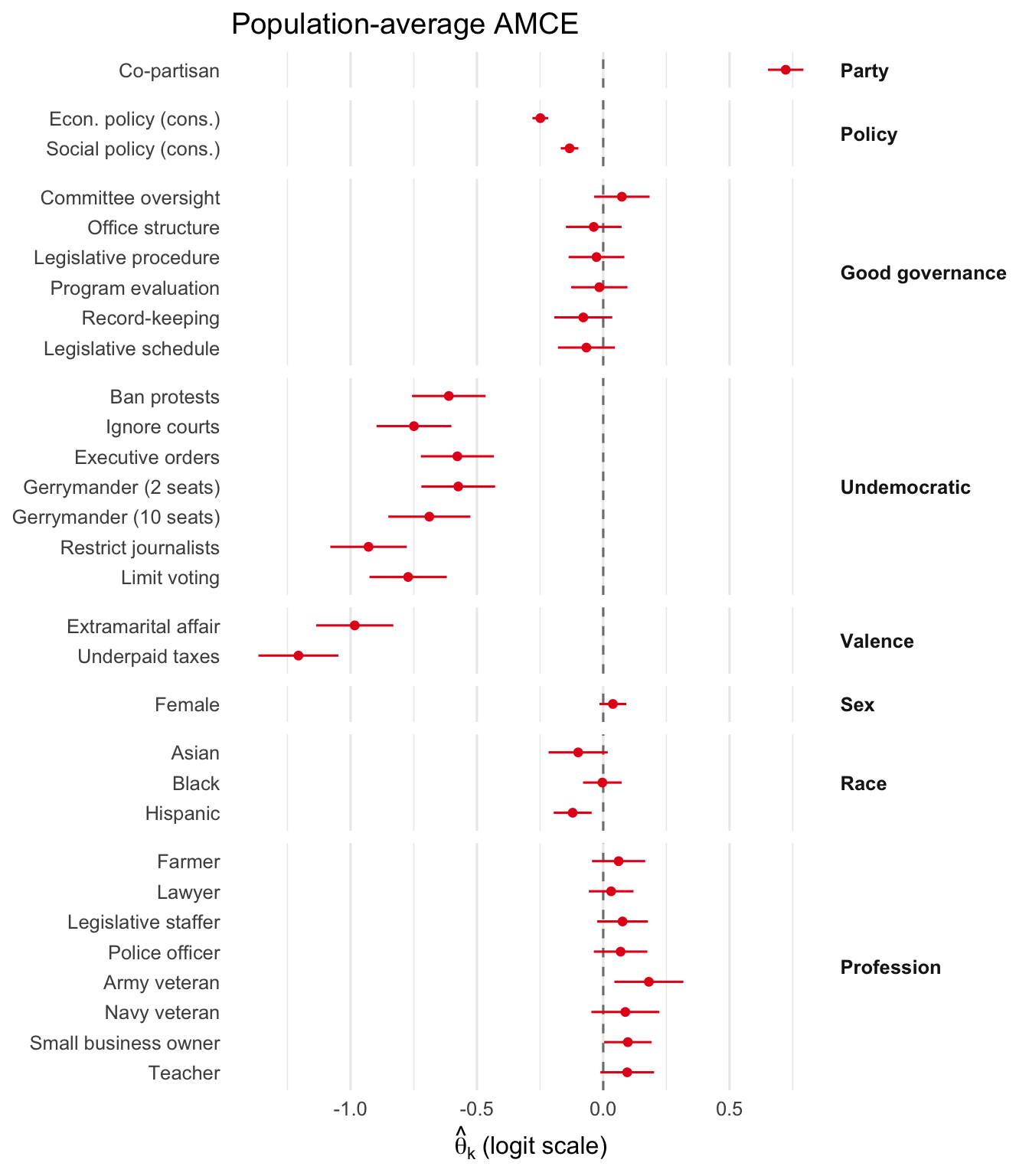
The population-average penalty for being a co-partisan candidate is a large, precisely-estimated positive coefficient (\(\hat\theta_{\text{co-partisan}} \approx +0.72\) on the logit scale), and every undemocratic action carries a strongly negative coefficient (range \(-0.57\) to \(-0.93\)). Restricting journalists is the most heavily penalized action (\(\hat\theta \approx -0.93\)); the valence scandals are even more damaging (extramarital affair \(\approx -0.98\)).

NoteThe Stage-2 default

scfit() runs an empirical-Bayes MAP refinement (paper EnsC5) on top of the Stage-1 DNN by default (stage2 = "map_c5"); the summary above reports it as Stage 2: map_c5. The DML population coefficients \(\hat\theta_k\) (the co-partisan and undemocratic-action effects above) and their clustered standard errors continue to use the Stage-1 single-DNN prediction (stored on fit_gs$beta_hat_dnn). The refined betas (fit_gs$beta_hat, with the respondent-indexed copy on fit_gs$beta_hat_resp) feed every distributional and individual-level quantity below. Set stage2 = "none" to recover the unrefined behaviour, or stage2 = "mixed_logit" for the BLUP alternative from the paper’s Supplementary Materials. Chapter 9 documents the full set of Stage-2 options.

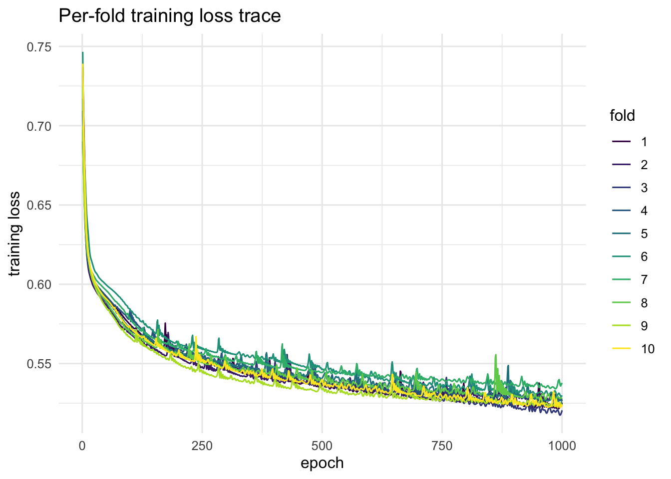
plot(fit_gs, "loss_trace")

3.3 Population-average estimates

NoteHow to read the AMCE plot

All dem_code contrasts are read relative to their absent / no-scandal baseline:

  • g_* (good-governance) items: near zero — voters are largely indifferent across procedural good-governance features.
  • u_* (undemocratic) items: strongly negative — voters penalize every undemocratic action.
  • v_* (valence violation) items: most negative — voters reject affairs and tax evasion most sharply.

This is the paper’s directional finding: voters broadly oppose democratic backsliding.

Plot the population-average coefficients (DML on the logit scale).

plot_amce(fit_gs, groups = gs_groups, labels = gs_labels)

3.3.1 Structural AME vs reduced-form AMCE

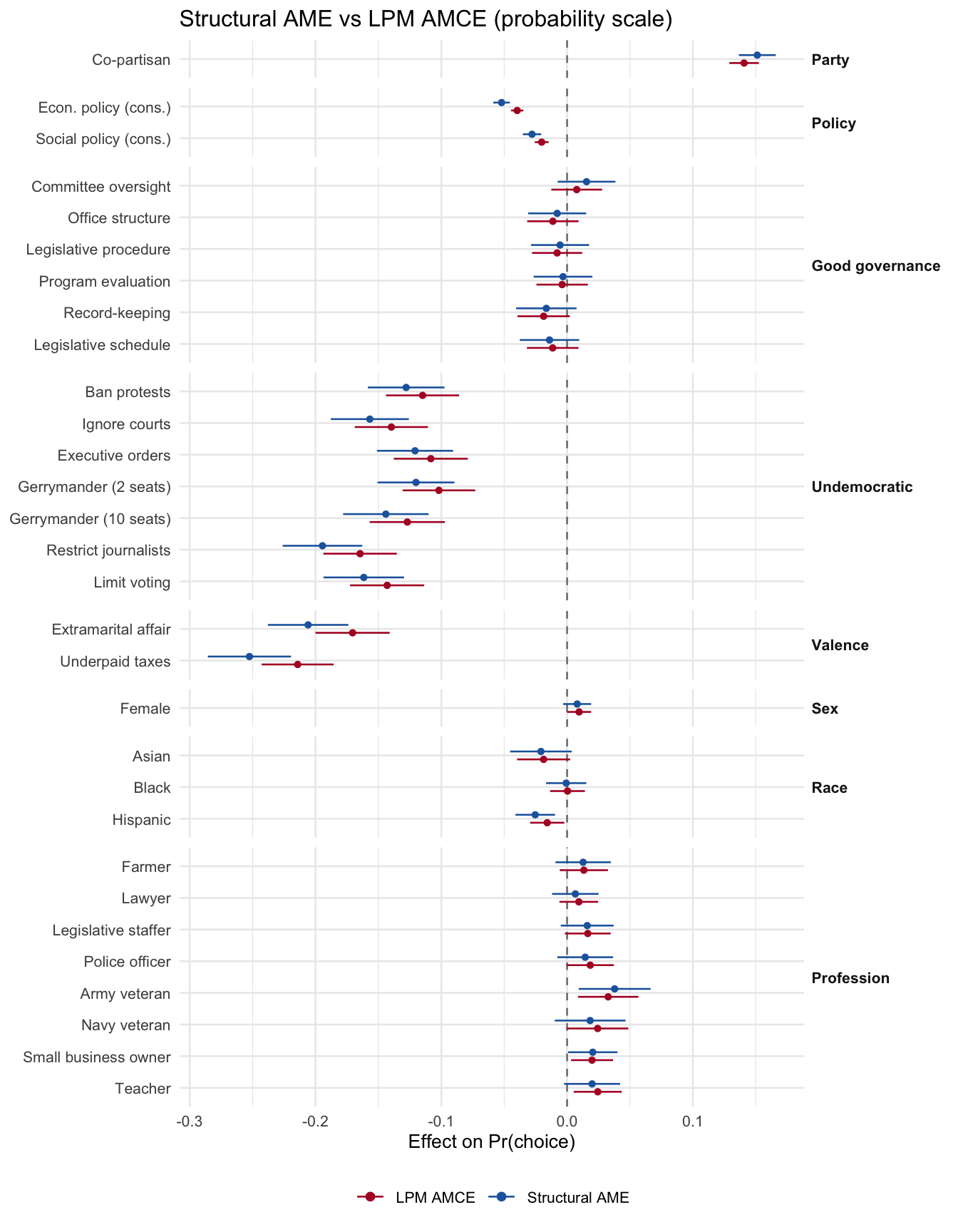
Overlay the structural model’s average marginal effects (probability scale) against the linear-probability-model AMCE. Under correct specification the two coincide.

ame_struct <- sc_average(fit_gs, scale = "probability")
ame_df     <- ame_struct$estimate; ame_df$source <- "Structural AME"
lpm        <- sc_baseline_lpm(fit_gs)
amce_df    <- data.frame(
  dummy_name = names(stats::coef(lpm)),
  estimate   = unname(stats::coef(lpm)),
  se         = sqrt(diag(stats::vcov(lpm))),
  source     = "LPM AMCE",
  stringsAsFactors = FALSE
)
amce_df$ci_lo <- amce_df$estimate - 1.96 * amce_df$se
amce_df$ci_hi <- amce_df$estimate + 1.96 * amce_df$se
df_both <- rbind(
  ame_df[, c("dummy_name", "estimate", "se", "ci_lo", "ci_hi", "source")],
  amce_df[, c("dummy_name", "estimate", "se", "ci_lo", "ci_hi", "source")]
)
df_both$label <- ifelse(df_both$dummy_name %in% names(gs_labels),
                        gs_labels[df_both$dummy_name],
                        df_both$dummy_name)
df_both$label <- factor(df_both$label,
                        levels = rev(intersect(unname(gs_labels), df_both$label)))
df_both$group <- gs_groups[df_both$dummy_name]
df_both$group <- factor(df_both$group, levels = unique(gs_groups))
df_both <- df_both[!is.na(df_both$group), ]

ggplot(df_both, aes(x = estimate, y = label, color = source)) +
  geom_vline(xintercept = 0, linetype = "dashed", color = "gray50") +
  geom_pointrange(aes(xmin = ci_lo, xmax = ci_hi),
                  position = position_dodge(width = 0.5),
                  size = 0.3, fatten = 2) +
  scale_color_manual(values = c("Structural AME" = "#2166AC",
                                "LPM AMCE"        = "#B2182B")) +
  facet_grid(group ~ ., scales = "free_y", space = "free_y") +
  labs(x = "Effect on Pr(choice)",
       y = NULL, color = NULL,
       title = "Structural AME vs LPM AMCE (probability scale)") +
  theme_minimal(base_size = 10) +
  theme(legend.position = "bottom",
        strip.text.y    = element_text(angle = 0, hjust = 0, face = "bold"))

3.4 Individual-level preferences

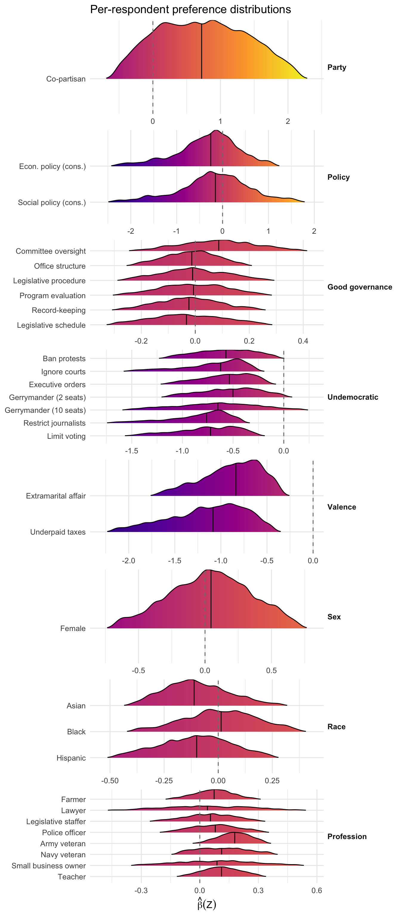
Ridgeline densities show how each per-respondent coefficient \(\hat\beta_k(\mathbf Z_i)\) is distributed across the sample. The undemocratic-action densities sit clearly left of zero for nearly every respondent — opposition to backsliding is broad, not confined to a subgroup — while the valence densities sit furthest left (see the callout above).

plot(fit_gs, "beta_ridgelines", groups = gs_groups, labels = gs_labels)

3.5 Structural quantities

3.5.1 Attribute importance

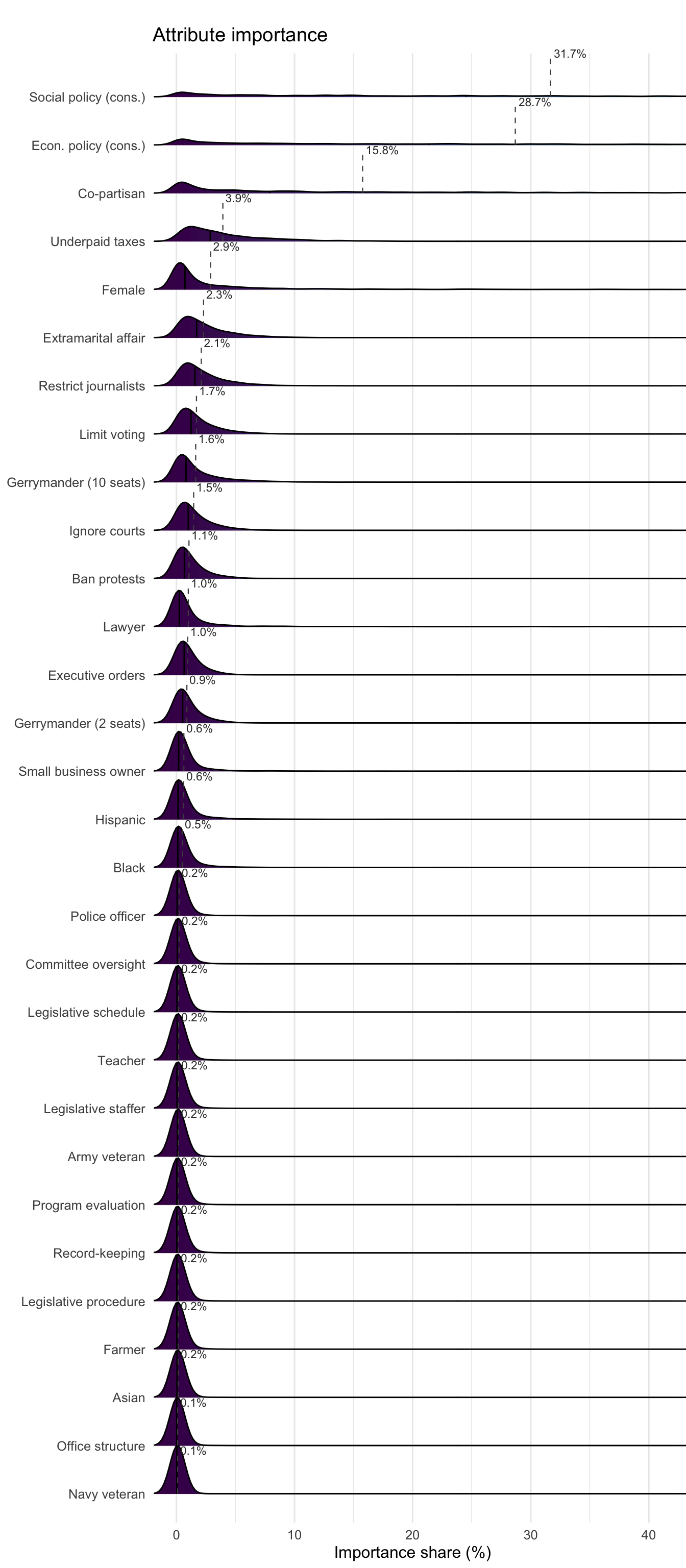
Decompose utility variance by attribute group. The package’s sc_importance() reports a per-contrast share; the paper groups the contrasts into attributes (party, policy, the three democracy families, and the candidate demographics) and reports the variance share of each attribute. Computing the grouped shares from the recovered per-respondent coefficients reproduces the paper’s decomposition.

B <- fit_gs$beta_hat_resp
attr_groups <- list(
  party    = "diff_respParty",
  policy   = c("diff_p1_num", "diff_p2_num"),
  good     = grep("_g_", colnames(B), value = TRUE),
  undem    = grep("_u_", colnames(B), value = TRUE),
  valence  = grep("_v_", colnames(B), value = TRUE),
  sex      = "diff_sex_Female",
  race     = grep("^diff_race_", colnames(B), value = TRUE),
  prof     = grep("^diff_pro_", colnames(B), value = TRUE)
)
## Per-respondent utility-variance per attribute over uniform level draws
## (reference contributes beta = 0, so L = #contrasts + 1).
imp <- sapply(attr_groups, function(cols) {
  ba <- B[, cols, drop = FALSE]; L <- ncol(ba) + 1
  rowSums(ba^2) / L - (rowSums(ba) / L)^2
})
shares <- 100 * colMeans(imp / rowSums(imp))
round(sort(shares, decreasing = TRUE), 1)
valence  policy   party   undem     sex    prof    race    good 
   29.4    26.1    23.1     9.2     4.3     3.1     3.0     1.8 

The leading shares are valence (\(\approx 29\%\)), policy (\(\approx 26\%\)), and party (\(\approx 23\%\)) clustered at the top, with the undemocratic-action attribute (\(\approx 9\%\)) carrying a smaller but non-trivial share. Voters care most about scandal, policy, and party; the democracy dimension matters, but it is not what most differentiates candidates in this design.

The package’s per-contrast view (uniform design) is complementary — it shows which individual contrasts within each attribute carry the variance:

sc_importance(fit_gs, design = "uniform")$estimate[, c("attribute", "share")]
                         attribute       share
1                   diff_respParty 0.115917186
2                      diff_p1_num 0.076994365
3                      diff_p2_num 0.089285682
4        diff_dem_code_g_committee 0.003741053
5  diff_dem_code_g_officestructure 0.001840055
6        diff_dem_code_g_procedure 0.002885534
7         diff_dem_code_g_progEval 0.002648745
8           diff_dem_code_g_record 0.002976534
9         diff_dem_code_g_schedule 0.003601388
10      diff_dem_code_u_banProtest 0.039828954
11           diff_dem_code_u_court 0.057544309
12        diff_dem_code_u_execRule 0.036386235
13          diff_dem_code_u_gerry2 0.031913740
14         diff_dem_code_u_gerry10 0.058546751
15     diff_dem_code_u_journalists 0.087438391
16       diff_dem_code_u_limitVote 0.066172906
17          diff_dem_code_v_affair 0.091095995
18             diff_dem_code_v_tax 0.153411363
19                 diff_sex_Female 0.020273085
20                 diff_race_Asian 0.004601456
21                 diff_race_Black 0.006122281
22              diff_race_Hispanic 0.007378772
23                 diff_pro_Farmer 0.002604294
24                 diff_pro_Lawyer 0.009474145
25    diff_pro_Legislative_staffer 0.003265660
26         diff_pro_Police_officer 0.004011984
27     diff_pro_Served_in_the_army 0.006014225
28     diff_pro_Served_in_the_navy 0.002934830
29   diff_pro_Small_business_owner 0.007613311
30                diff_pro_Teacher 0.003476770
plot_importance(fit_gs, labels = gs_labels, xlim = c(0, 40))

3.6 Heterogeneity test

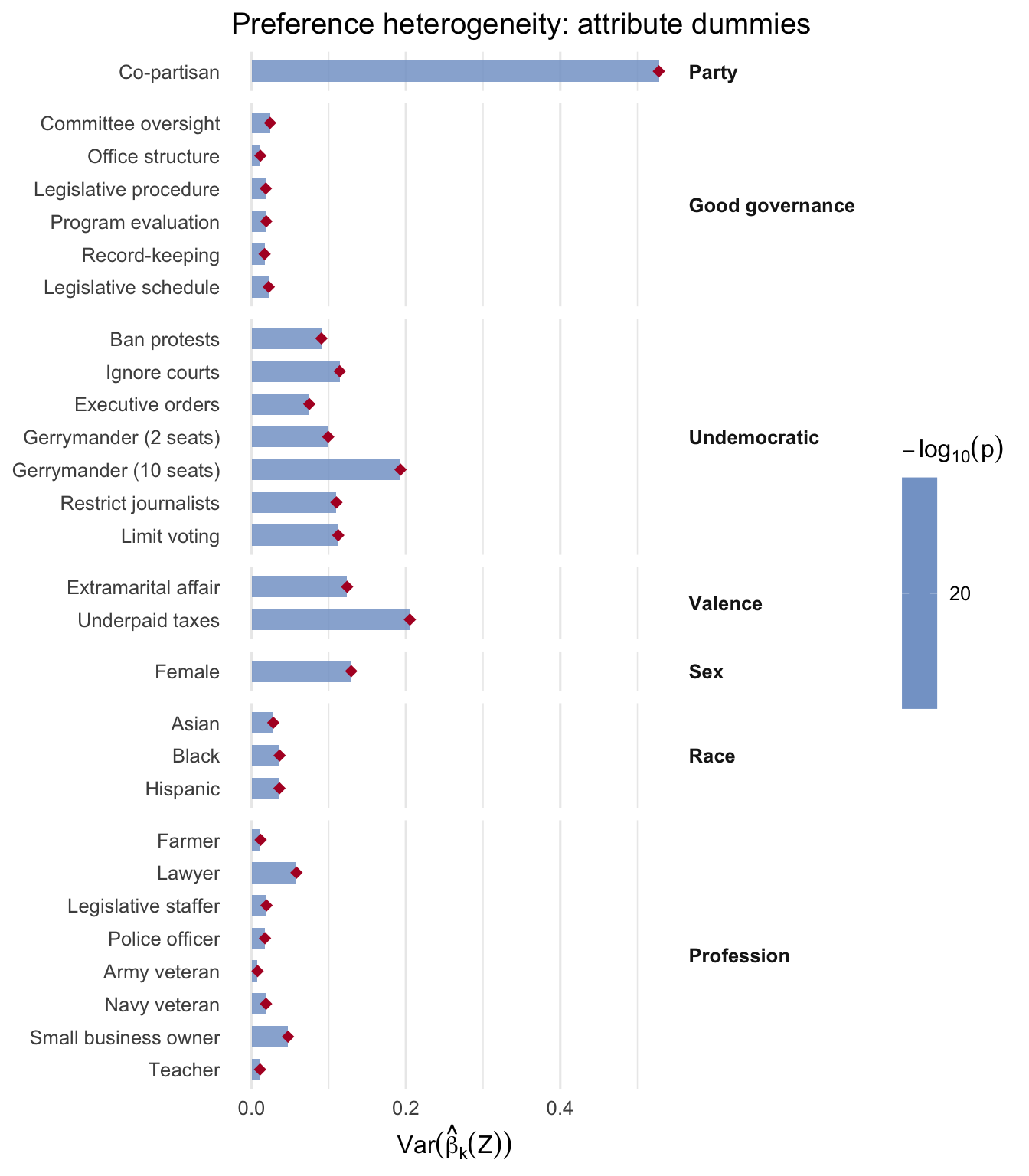
Does the per-attribute dispersion of \(\hat\beta_k(\mathbf Z_i)\) exceed what sampling noise alone would explain? A significant result for the u_* levels confirms that the intensity of the penalty for undemocratic behavior varies meaningfully across respondents.

het_gs <- sc_heterogeneity_test(fit_gs, adjust = "bh")
het_gs$estimate
                        dummy_name     var_beta       se_var    t_stat
1                   diff_respParty  0.527742363 0.0177695771 29.699208
2                      diff_p1_num 15.670804678 4.6800046661  3.348459
3                      diff_p2_num 21.346131631 5.8350805813  3.658241
4        diff_dem_code_g_committee  0.023995414 0.0011899264 20.165460
5  diff_dem_code_g_officestructure  0.011401571 0.0004269150 26.706886
6        diff_dem_code_g_procedure  0.018455676 0.0006629046 27.840620
7         diff_dem_code_g_progEval  0.019079375 0.0007254185 26.301196
8           diff_dem_code_g_record  0.016878679 0.0006462544 26.117701
9         diff_dem_code_g_schedule  0.022226129 0.0007595945 29.260519
10      diff_dem_code_u_banProtest  0.090533973 0.0027259576 33.211805
11           diff_dem_code_u_court  0.114215885 0.0045508374 25.097773
12        diff_dem_code_u_execRule  0.074784651 0.0025884053 28.892172
13          diff_dem_code_u_gerry2  0.099303679 0.0031111824 31.918309
14         diff_dem_code_u_gerry10  0.192996961 0.0064711666 29.824137
15     diff_dem_code_u_journalists  0.109943574 0.0044635890 24.631205
16       diff_dem_code_u_limitVote  0.112287327 0.0039601153 28.354560
17          diff_dem_code_v_affair  0.123802513 0.0045264192 27.351093
18             diff_dem_code_v_tax  0.205138942 0.0071791959 28.574083
19                 diff_sex_Female  0.129108113 0.0066820067 19.321758
20                 diff_race_Asian  0.028113643 0.0010631883 26.442769
21                 diff_race_Black  0.036292681 0.0013512672 26.858256
22              diff_race_Hispanic  0.036072012 0.0015623797 23.087866
23                 diff_pro_Farmer  0.011701826 0.0004655026 25.138049
24                 diff_pro_Lawyer  0.058195232 0.0021806859 26.686664
25    diff_pro_Legislative_staffer  0.019319257 0.0007157211 26.992716
26         diff_pro_Police_officer  0.017370829 0.0006513586 26.668612
27     diff_pro_Served_in_the_army  0.007754411 0.0002800981 27.684627
28     diff_pro_Served_in_the_navy  0.018731826 0.0005623285 33.311179
29   diff_pro_Small_business_owner  0.047230039 0.0016179405 29.191456
30                diff_pro_Teacher  0.010968817 0.0003940687 27.834780
         p_value    p_adjusted sig
1  3.930808e-194 2.358485e-193 ***
2   4.063112e-04  4.063112e-04 ***
3   1.269760e-04  1.313545e-04 ***
4   9.845320e-91  1.093924e-90 ***
5  1.957594e-157 3.454578e-157 ***
6  6.995500e-171 1.907864e-170 ***
7  9.291281e-153 1.327326e-152 ***
8  1.147504e-150 1.564779e-150 ***
9  1.649832e-188 8.249158e-188 ***
10 3.635815e-242 5.453722e-241 ***
11 2.629817e-139 3.287271e-139 ***
12 7.486774e-184 2.807540e-183 ***
13 7.439052e-224 7.439052e-223 ***
14 9.504026e-196 7.128019e-195 ***
15 2.926157e-134 3.511388e-134 ***
16 3.676886e-177 1.103066e-176 ***
17 5.240248e-165 1.122910e-164 ***
18 7.053594e-180 2.351198e-179 ***
19  1.762217e-83  1.888090e-83 ***
20 2.209446e-154 3.314169e-154 ***
21 3.377674e-159 6.333138e-159 ***
22 3.065338e-118 3.536929e-118 ***
23 9.547305e-140 1.245301e-139 ***
24 3.361331e-157 5.602219e-157 ***
25 8.997693e-161 1.799539e-160 ***
26 5.444484e-157 8.596554e-157 ***
27 5.346627e-169 1.233837e-168 ***
28 1.329916e-243 3.989747e-242 ***
29 1.244667e-187 5.334289e-187 ***
30 8.232138e-171 2.058034e-170 ***

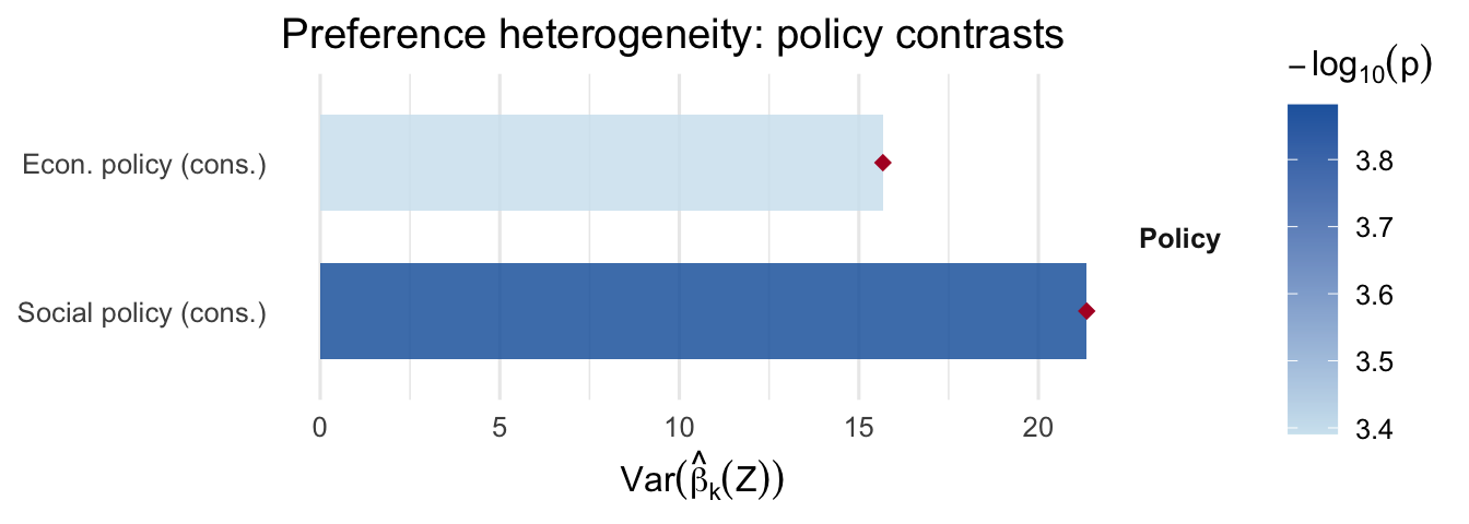
The two policy contrasts are continuous (a 1–4 conservatism scale), so their coefficient variances are far larger than those of the binary attribute dummies and would compress every other bar onto an unreadable scale. We plot the dummies and the two policy contrasts separately.

policy_contrasts <- c("diff_p1_num", "diff_p2_num")
plot_hetero(fit_gs,
            dummies = setdiff(fit_gs$attr_names, policy_contrasts),
            groups = gs_groups, labels = gs_labels,
            title = "Preference heterogeneity: attribute dummies")

plot_hetero(fit_gs, dummies = policy_contrasts,
            groups = gs_groups, labels = gs_labels,
            title = "Preference heterogeneity: policy contrasts")

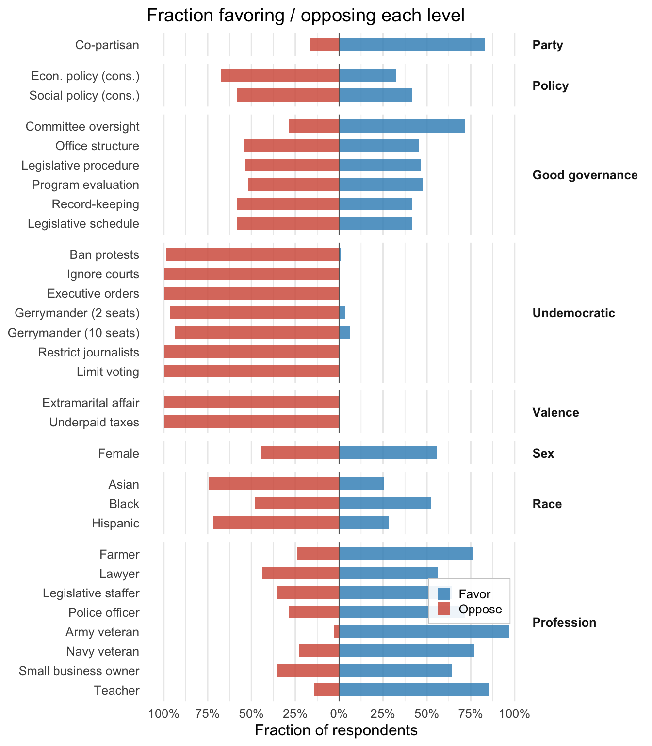
The penalty for each undemocratic action varies in intensity across respondents, but its population average is strongly negative for every action: on average, voters oppose democratic backsliding. The opposition is also broad at the individual level — the next section shows that almost no respondents actively favor any undemocratic action.

3.6.1 Fraction preferring

fr <- sc_fraction_preferring(fit_gs)
fr_u <- fr$estimate[grepl("^diff_dem_code_u_", fr$estimate$dummy_name), ]
fr_u$action <- sub("diff_dem_code_u_", "", fr_u$dummy_name)
round(setNames(fr_u$frac_positive, fr_u$action), 3)
 banProtest       court    execRule      gerry2     gerry10 journalists 
      0.011       0.000       0.002       0.034       0.061       0.000 
  limitVote 
      0.000 

The fraction of respondents who actively favor any undemocratic action is tiny. The least-opposed action, a 10-seat gerrymander, is favored by only about 6% of respondents — over 93% are opposed — and restricting journalists, ignoring courts, and limiting voting are favored by essentially no one. This is the paper’s individual-level finding: opposition to undemocratic behavior is nearly universal, not a property of one partisan camp.

plot_fraction(fit_gs, groups = gs_groups, labels = gs_labels)

3.7 Direction and intensity

The undemocratic levels show a large negative average direction (voters penalize them) coupled with high intensity. The structural question is whether the dispersion of those coefficients concentrates on co-partisans, as Graham and Svolik argue.

sc_direction_intensity(fit_gs)
sc_quantity_bivariate: direction_intensity
-- direction --
sc_quantity: direction
  estimate: data.frame with 30 rows
                      dummy_name        d     se_d  ci_lo_d   ci_hi_d
                  diff_respParty  0.66588 0.018685  0.62925  0.702498
                     diff_p1_num -0.34579 0.023478 -0.39181 -0.299775
                     diff_p2_num -0.16338 0.024679 -0.21175 -0.115012
       diff_dem_code_g_committee  0.43051 0.022592  0.38623  0.474788
 diff_dem_code_g_officestructure -0.09038 0.024916 -0.13922 -0.041546
       diff_dem_code_g_procedure -0.06889 0.024959 -0.11780 -0.019969
        diff_dem_code_g_progEval -0.04129 0.024999 -0.09029  0.007703
          diff_dem_code_g_record -0.16387 0.024679 -0.21224 -0.115498
        diff_dem_code_g_schedule -0.16406 0.024670 -0.21241 -0.115708
      diff_dem_code_u_banProtest -0.97734 0.005311 -0.98775 -0.966935
  ... 20 more rows
-- intensity --
sc_quantity: intensity
  estimate: data.frame with 30 rows
                      dummy_name       u     se_u ci_lo_u ci_hi_u
                  diff_respParty 0.84163 0.015137 0.81196 0.87129
                     diff_p1_num 1.03062 0.095871 0.84272 1.21853
                     diff_p2_num 1.14964 0.112471 0.92920 1.37008
       diff_dem_code_g_committee 0.14032 0.002707 0.13502 0.14563
 diff_dem_code_g_officestructure 0.08529 0.001663 0.08203 0.08855
       diff_dem_code_g_procedure 0.10748 0.002086 0.10339 0.11157
        diff_dem_code_g_progEval 0.11005 0.002097 0.10594 0.11416
          diff_dem_code_g_record 0.10397 0.002041 0.09997 0.10797
        diff_dem_code_g_schedule 0.12245 0.002228 0.11808 0.12681
      diff_dem_code_u_banProtest 0.58360 0.007448 0.56900 0.59820
  ... 20 more rows

3.7.1 Marginal rate of substitution: democracy vs party

How much co-partisan advantage would a candidate need to offset the penalty for an undemocratic action? The population MRS is the ratio of the action’s coefficient to the co-partisan coefficient, \(\theta_{\text{action}} / \theta_{\text{co-partisan}}\), estimated with the debiased orthogonal score (estimand = "population").

mrs_actions <- c("diff_dem_code_u_journalists",
                 "diff_dem_code_u_court",
                 "diff_dem_code_u_gerry10")
do.call(rbind, lapply(mrs_actions, function(a) {
  m <- sc_mrs(fit_gs, a, "diff_respParty", estimand = "population")
  data.frame(action = sub("diff_dem_code_u_", "", a),
             abs_mrs = round(abs(m$estimate), 2),
             se      = round(m$se, 2),
             row.names = NULL)
}))
       action abs_mrs   se
1 journalists    1.29 0.12
2       court    1.04 0.12
3     gerry10    0.95 0.12

Restricting journalists costs about 1.3 co-partisan-advantages to offset; ignoring courts about 1.0; a 10-seat gerrymander about 0.95. In words, a candidate would have to be more than a co-partisan — worth roughly 1.3 party switches — to make the average voter forgive prosecuting journalists. Party loyalty does not buy a free pass on the most severe undemocratic actions.

3.8 Subgroup analysis by partisanship

We re-average the held-out \(\hat\beta(\mathbf Z_i)\) separately for Democrats, Independents, and Republicans using sc_subgroup(). The convenience column pid7 carries the raw 7-point party identification (\(<0\) Democrat, \(0\) Independent, \(>0\) Republican). sc_subgroup() expects a logical vector aligned to the fit’s task rows (one per respondent–task), so we map the respondent-level pid7 onto fit_gs$respondent_id.

## Respondent-level lookups, indexed onto the fit's task rows.
pid_lookup  <- tapply(gs2020$pid7,  gs2020$respondent, function(x) x[1])
ideo_lookup <- tapply(gs2020$ideo7, gs2020$respondent, function(x) x[1])
rid       <- as.character(fit_gs$respondent_id)
pid_row   <- unname(pid_lookup[rid])    # length = nrow(fit_gs$beta_hat)
ideo_row  <- unname(ideo_lookup[rid])
sub <- sc_subgroup(fit_gs, list(
  Democrat    = pid_row < 0,
  Independent = pid_row == 0,
  Republican  = pid_row > 0
))
do.call(rbind, lapply(names(sub), function(g) {
  e <- sub[[g]]$estimate
  rows <- grepl("^diff_dem_code_u_", e$dummy_name)
  data.frame(group = g, action = sub("diff_dem_code_u_", "", e$dummy_name[rows]),
             theta = round(e$theta[rows], 2), se = round(e$se[rows], 2),
             row.names = NULL)
}))
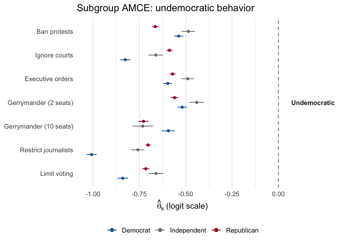
         group      action theta   se
1     Democrat  banProtest -0.54 0.01
2     Democrat       court -0.83 0.01
3     Democrat    execRule -0.60 0.01
4     Democrat      gerry2 -0.52 0.01
5     Democrat     gerry10 -0.59 0.02
6     Democrat journalists -1.01 0.01
7     Democrat   limitVote -0.84 0.01
8  Independent  banProtest -0.49 0.02
9  Independent       court -0.66 0.02
10 Independent    execRule -0.49 0.02
11 Independent      gerry2 -0.44 0.02
12 Independent     gerry10 -0.73 0.03
13 Independent journalists -0.76 0.02
14 Independent   limitVote -0.66 0.02
15  Republican  banProtest -0.66 0.01
16  Republican       court -0.59 0.01
17  Republican    execRule -0.57 0.01
18  Republican      gerry2 -0.56 0.01
19  Republican     gerry10 -0.73 0.01
20  Republican journalists -0.70 0.01
21  Republican   limitVote -0.72 0.01
plot_subgroup(
  fit_gs,
  subgroup = list(Democrat    = pid_row < 0,
                  Independent = pid_row == 0,
                  Republican  = pid_row > 0),
  dummies = grep("^diff_dem_code_u_", fit_gs$attr_names, value = TRUE),
  groups = gs_groups, labels = gs_labels,
  title = "Subgroup AMCE: undemocratic behavior"
)

The structural model reveals that strong partisans of both parties penalize undemocratic behavior; the intensity of the penalty varies across respondents, but its sign does not. We can sharpen this with ideology terciles, built from the raw 7-point ideology column ideo7 (1–3 Liberal, 4 Moderate, 5–7 Conservative), again indexed onto the task rows via ideo_row:

ideo_grp <- cut(ideo_row, c(0, 3, 4, 7),
                labels = c("Liberal", "Moderate", "Conservative"))
sub_ideo <- sc_subgroup(fit_gs, list(
  Liberal      = ideo_grp == "Liberal",
  Moderate     = ideo_grp == "Moderate",
  Conservative = ideo_grp == "Conservative"
))
do.call(rbind, lapply(names(sub_ideo), function(g) {
  e <- sub_ideo[[g]]$estimate
  i <- e$dummy_name == "diff_dem_code_u_journalists"
  data.frame(ideology = g, action = "journalists",
             theta = round(e$theta[i], 2), se = round(e$se[i], 2),
             row.names = NULL)
}))
      ideology      action theta   se
1      Liberal journalists -1.10 0.02
2     Moderate journalists -0.78 0.01
3 Conservative journalists -0.69 0.01

Every ideological tercile assigns a strong negative coefficient to restricting journalists: the penalty is broad across the ideological spectrum.

3.9 Preference clustering

A complementary view on latent preference types: run k-means on the per-respondent \(\hat\beta(\mathbf Z_i)\) matrix to find clusters of respondents with similar preference profiles.

cl_gs <- sc_clusters(fit_gs, k = 3L, seed = 2024)
cl_gs$estimate$sizes
[1] 5041 7809 7807
round(cl_gs$estimate$centers, 2)
     diff_respParty diff_p1_num diff_p2_num diff_dem_code_g_committee
[1,]           0.94       -1.36       -1.15                      0.21
[2,]           0.88       -0.20        0.18                      0.08
[3,]           0.47       -0.38       -0.31                      0.01
     diff_dem_code_g_officestructure diff_dem_code_g_procedure
[1,]                            0.03                      0.05
[2,]                           -0.05                     -0.01
[3,]                           -0.01                     -0.04
     diff_dem_code_g_progEval diff_dem_code_g_record diff_dem_code_g_schedule
[1,]                    -0.01                   0.05                     0.12
[2,]                    -0.06                  -0.03                    -0.07
[3,]                     0.06                  -0.07                    -0.08
     diff_dem_code_u_banProtest diff_dem_code_u_court
[1,]                      -0.92                 -1.19
[2,]                      -0.66                 -0.62
[3,]                      -0.28                 -0.48
     diff_dem_code_u_execRule diff_dem_code_u_gerry2 diff_dem_code_u_gerry10
[1,]                    -0.93                  -0.92                   -1.18
[2,]                    -0.58                  -0.57                   -0.72
[3,]                    -0.33                  -0.22                   -0.28
     diff_dem_code_u_journalists diff_dem_code_u_limitVote
[1,]                       -1.30                     -1.22
[2,]                       -0.74                     -0.74
[3,]                       -0.66                     -0.49
     diff_dem_code_v_affair diff_dem_code_v_tax diff_sex_Female
[1,]                  -1.37               -1.77            0.08
[2,]                  -0.90               -1.15            0.01
[3,]                  -0.58               -0.76            0.04
     diff_race_Asian diff_race_Black diff_race_Hispanic diff_pro_Farmer
[1,]           -0.22           -0.01              -0.02            0.09
[2,]           -0.16            0.05              -0.17            0.07
[3,]            0.05           -0.01              -0.09            0.06
     diff_pro_Lawyer diff_pro_Legislative_staffer diff_pro_Police_officer
[1,]            0.11                         0.04                    0.00
[2,]            0.00                        -0.01                    0.13
[3,]            0.04                         0.11                    0.07
     diff_pro_Served_in_the_army diff_pro_Served_in_the_navy
[1,]                        0.16                        0.23
[2,]                        0.19                        0.16
[3,]                        0.18                       -0.01
     diff_pro_Small_business_owner diff_pro_Teacher
[1,]                          0.13             0.12
[2,]                          0.10             0.11
[3,]                          0.04             0.11

3.10 Validating against the homogeneous-logit AMCE

The structural model nests the standard pooled-logit AMCE: under correct logit specification, \(\theta_k = \mathbb{E}[\beta_k(Z)]\) equals the homogeneous-logit coefficient on attribute \(k\). The sc_validate_amce() export reports this comparison.

v_gs <- sc_validate_amce(fit_gs)
v_gs
sc_validate_amce -- pooled and (optionally) subgroup comparison
Stage 2: map_c5
N obs: 20657, N respondents: 1605, P attributes: 30
Pooled correlation (DML theta vs homogeneous logit coef): 0.999

Pooled comparison (first 10 rows):
                       attribute dml_theta dml_se homog_logit_coef
                  diff_respParty    0.7222 0.0358           0.6277
                     diff_p1_num   -0.2488 0.0160          -0.1779
                     diff_p2_num   -0.1331 0.0178          -0.0907
       diff_dem_code_g_committee    0.0739 0.0560           0.0337
 diff_dem_code_g_officestructure   -0.0376 0.0563          -0.0484
       diff_dem_code_g_procedure   -0.0267 0.0562          -0.0356
        diff_dem_code_g_progEval   -0.0155 0.0569          -0.0170
          diff_dem_code_g_record   -0.0789 0.0585          -0.0827
        diff_dem_code_g_schedule   -0.0668 0.0575          -0.0509
      diff_dem_code_u_banProtest   -0.6112 0.0742          -0.4995
 homog_logit_se     diff abs_diff
        0.00599  0.09457  0.09457
        0.00250 -0.07092  0.07092
        0.00281 -0.04239  0.04239
        0.01031  0.04020  0.04020
        0.01041  0.01081  0.01081
        0.01017  0.00889  0.00889
        0.01041  0.00156  0.00156
        0.01062  0.00378  0.00378
        0.01045 -0.01583  0.01583
        0.01482 -0.11170  0.11170

A correlation near \(r = 1\) across the 30 attribute levels confirms that nothing a reduced-form AMCE analysis would deliver is lost by using the structural model.

3.11 Summary

This application shows what the structural estimator adds beyond a reduced-form AMCE:

  • The population averages recover the familiar finding: voters of both parties penalize undemocratic behavior, and restricting journalists is the most heavily penalized undemocratic action.
  • Opposition is broad rather than universal. For every undemocratic action, all but a small minority of respondents place negative weight on it; what varies across respondents is the intensity of that opposition, not its direction.
  • Decomposing utility variance places valence, policy, and party near the top, with the democracy attribute below them.
  • The population marginal rate of substitution prices each violation against co-partisanship.

None of these quantities is available from one-attribute-at-a-time effects; each follows from the recovered preference vector \(\hat\beta_i(\mathbf Z)\).