The package also implements sensitivity tests to help researchers assess the strong and generally untestable exogeneity assumption. These tests apply to the just-identified (one-treatment-one-instrument) case.
Bound and Jaeger (2000) suggest zero-first-stage (ZFS) tests, which use an auxiliary regression on a subsample where the instrument is not expected to influence treatment assignment. A ZFS test can be understood as a placebo test. If there is a strong prior that the first stage is zero in a subsample, the reduced-form effect should also be zero if the exogeneity assumption holds. In the language of the LATE framework, this subsample has no compliers, only always-takers and never-takers.
Researchers first use substantive knowledge to identify a subsample in which the instrument’s first-stage effect is likely zero (henceforth, the ZFS subsample). They then regress \(Y\) on \(Z\) in this subsample to show that the reduced-form coefficient for the instrument is approximately zero. This provides suggestive evidence in favor of instrument validity. For most observational instruments, substantive knowledge of the assignment mechanism ought to identify a ZFS subsample.
We recommend this heuristic check for most observational IV papers. The reduced-form coefficient can be tested against zero, but failing to reject does not show that the exclusion restriction holds. Van Kippersluis and Rietveld (2018) demonstrate that the ZFS test can be usefully combined with the “plausibly exogenous” method suggested by Conley et al. (2012) (henceforth, CHR 2012). To illustrate the method, we rewrite the IV simultaneous equations in CHR (2012)’s notation:
where the instrument \(Z\) also enters the structural equation. The exclusion restriction amounts to a dogmatic prior that \(\gamma=0\). CHR (2012) suggest relaxing this assumption by specifying a plausible value, range, or distribution for \(\gamma\). This choice depends on the researcher’s beliefs about the degree of violation of the exclusion restriction. They propose three approaches to inference. The first specifies a range of values for \(\gamma\); the second specifies a prior distribution for \(\gamma\); the third is a fully Bayesian analysis that requires priors over all model parameters and corresponding parametric distributions.
We focus on the second method, which CHR (2012) call the local-to-zero (LTZ) approximation, because of its simplicity and transparency. The LTZ approximation considers “local” violations of the exclusion restriction and requires a prior over \(\gamma\) alone. CHR (2012) replace the standard assumption that \(\gamma = 0\) with the weaker assumption that \(\gamma
\sim \mathbb{F}\), a prior distribution. They show that this implies the following distribution of \(\hat\beta\): \[
\hat{\beta} \sim^a N(\beta, \mathbb{V}_{2SLS}) + A \gamma
\] where \(A = (X'Z(Z'Z)^{-1}Z'X)^{-1} X'Z\). The additional term inflates the original 2SLS asymptotic distribution. With a Gaussian prior over \(\gamma \sim N(\mu_\gamma, \Omega_\gamma)\), the distribution takes its most convenient form. In this case, \(\hat\beta\) is approximately normal with mean \(\beta + A \mu_\gamma\): \[
\hat{\beta} \sim^a N(\beta + A \mu_\gamma ,
\mathbb{V}_{2SLS} + A \Omega_\gamma A')
\] In practice, researchers can replace \(\mu_\gamma\) with an estimate from the ZFS and \(\Omega_\gamma\) with the estimate’s estimated variance. The LTZ estimate is then \(\hat\beta - A\hat\mu_\gamma\), with variance \(\mathbb{V}_{2SLS} + A\hat\Omega_\gamma A'\); ltz() reports both.
5.1 The persistence of social capital
We illustrate the diagnostics with the IV analysis in Guiso et al. (2016) (henceforth GSZ 2016). They revisit Putnam et al. (1993)’s celebrated conjecture that Italian cities that achieved self-government in the Middle Ages have higher modern-day levels of social capital. They study the effects of free city-state status on social capital using measures of the number of nonprofit organizations per capita, organ donations per capita, and whether students cheat in mathematics. This tutorial focuses on the first outcome. The table below summarizes the analysis.
Summary
Unit of analysis
Italian city
Treatment
historical free city status
Instrument
whether a city was the seat of a bishop in the Middle Ages
Outcome
the number of nonprofit organizations per capita
Model
Table 6
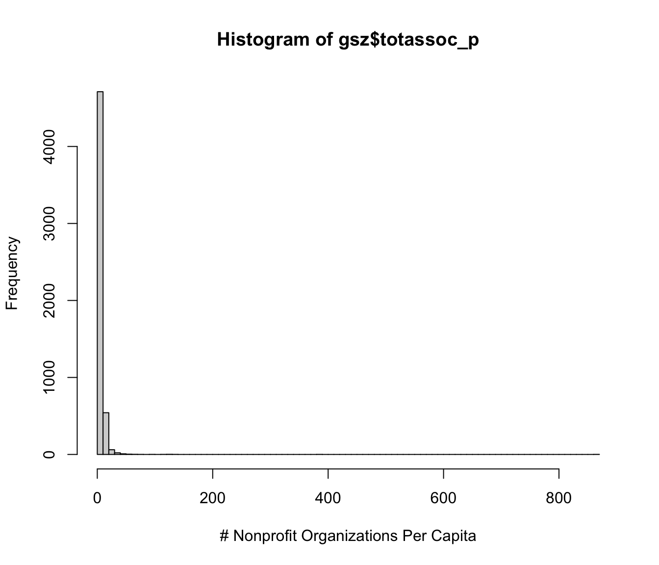
First, identify the key variables in the replication data and examine their distributions. The outcome variable is highly skewed, but we keep it unchanged to be consistent with the original paper.
library(ivDiag)Y<-"totassoc_p"D<-"libero_comune_allnord"Z<-"bishopcity"weights<-"population"controls<-c('altitudine', 'escursione', 'costal', 'nearsea', 'population', 'pop2', 'gini_land', 'gini_income')# table instrument and treatmenttable(gsz$bishopcity)#> #> 0 1 #> 5178 179table(gsz$libero_comune_allnord)#> #> 0 1 #> 5293 64table(gsz$bishopcity, gsz$libero_comune_allnord)#> #> 0 1#> 0 5173 5#> 1 120 59# distribution of the outcomehist(gsz$totassoc_p, breaks =100, xlab ="# Nonprofit Organizations Per Capita")
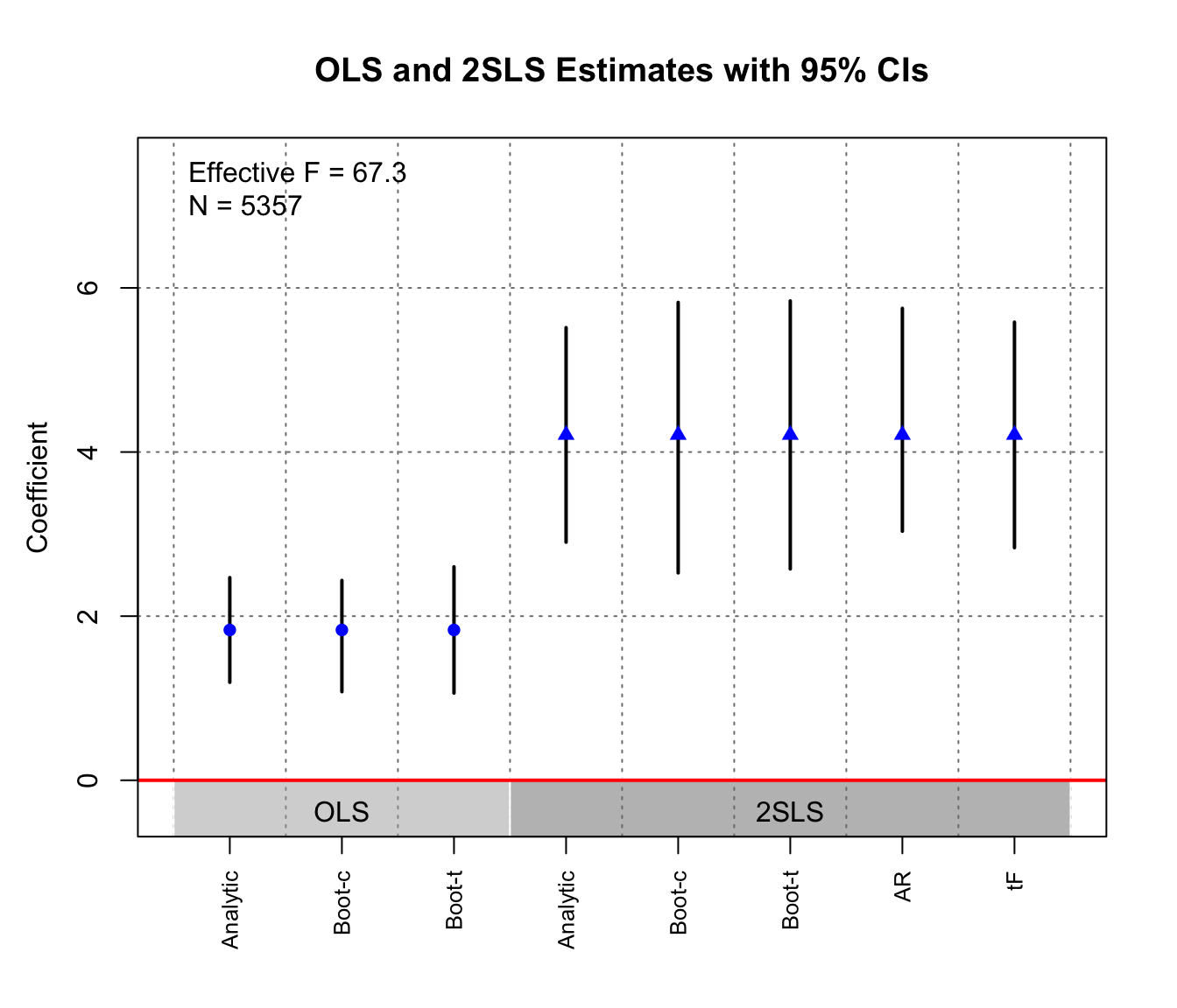
Apply the omnibus function ivDiag, then plot the OLS and 2SLS coefficients and corresponding CIs.
The results show that the 2SLS estimates are larger in magnitude than the OLS estimates. Different inferential methods for the 2SLS estimates produce slightly different CIs, but all reject the null of no effect quite comfortably.
The authors conduct a ZFS test using the subsample of southern Italian cities, where the free-city experience was arguably irrelevant. The ZFS test is simply a reduced-form regression of the outcome on the instrument. The coefficient and SE of the instrument bishopcity are 0.178 and 0.137, respectively.
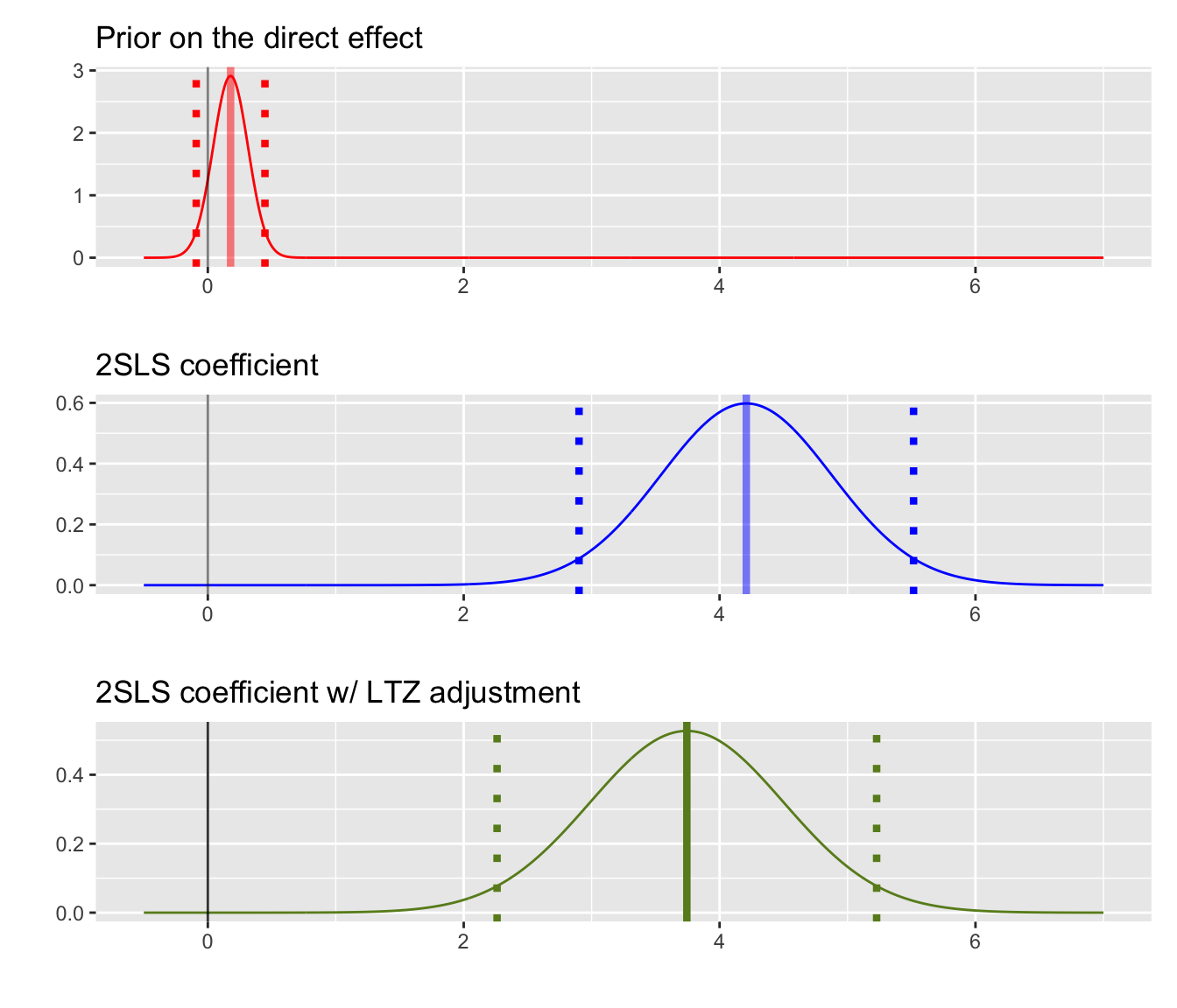
To perform an LTZ adjustment on the 2SLS/IV estimate, set the prior mean to 0.178 and its standard deviation (SD) to 0.137.
ltz_out<-ltz(data =gsz, Y =Y, D =D, Z =Z, controls =controls, weights =weights, prior =c(0.178, 0.137))ltz_out#> $iv#> Coef SE t CI 2.5% CI 97.5% p-value #> 4.2087 0.6670 6.3097 2.9014 5.5160 0.0000 #> #> $ltz#> Coef SE t CI 2.5% CI 97.5% p-value #> 3.7441 0.7568 4.9471 2.2607 5.2275 0.0000 #> #> $prior#> Mean SD #> 0.178 0.137 #> #> attr(,"class")#> [1] "ltz"
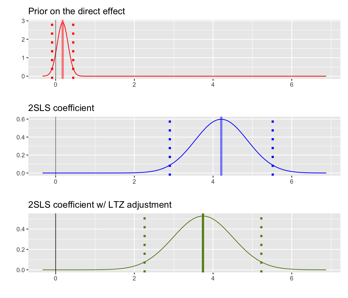
Pass the output from ltz to plot_ltz to plot the approximate sampling distribution of the 2SLS estimates before and after LTZ adjustment. The plot also shows the prior distribution based on the ZFS test. The dotted lines mark 95% intervals: the central 95% of the prior in the first panel, and the 95% CIs of the estimates in the other two. In this case, the original finding remains robust to the LTZ adjustment.
Alternatively, pass the IV estimates, the LTZ estimates, and the prior separately to plot_ltz. Each input is a two-element vector containing a coefficient and an SD/SE estimate.
Bound, John, and David A Jaeger. 2000. “Do Compulsory School Attendance Laws Alone Explain the Association Between Quarter of Birth and Earnings?” In Research in Labor Economics, vol. 19. Emerald Group Publishing Limited.
Conley, Timothy G, Christian B Hansen, and Peter E Rossi. 2012. “Plausibly Exogenous.”Review of Economics and Statistics 94 (1): 260–72.
Guiso, Luigi, Paola Sapienza, and Luigi Zingales. 2016. “Long-Term Persistence.”Journal of the European Economic Association 14 (6): 1401–36.
Putnam, Robert D, Robert Leonardi, and Raffaella Y Nanetti. 1993. Making Democracy Work: Civic Traditions in Modern Italy. Princeton University Press.
Van Kippersluis, Hans, and Cornelius A Rietveld. 2018. “Beyond Plausibly Exogenous.”The Econometrics Journal 21 (3): 316–31.
Source Code
# Sensitivity Tests {#sec-sensitivity}```{r setup, include = FALSE}knitr::opts_chunk$set(echo =TRUE, cache =TRUE)```The package also implements sensitivity tests to help researchers assess the strong and generally untestable exogeneity assumption. These tests apply to the **just-identified** (one-treatment-one-instrument) case. @bound2000compulsory suggest **zero-first-stage** (ZFS) tests, which use an auxiliary regression on a subsample where the instrument is not expected to influence treatment assignment. A ZFS test can be understood as a placebo test. If there is a strong prior that the first stage is zero in a subsample, the reduced-form effect should also be zero if the exogeneity assumption holds. In the language of the LATE framework, this subsample has no compliers, only always-takers and never-takers.Researchers first use substantive knowledge to identify a subsample in which the instrument's first-stage effect is likely zero (henceforth, the ZFS subsample). They then regress $Y$ on $Z$ in this subsample to show that the reduced-form coefficient for the instrument is approximately zero. This provides suggestive evidence in favor of instrument validity. For most observational instruments, substantive knowledge of the assignment mechanism ought to identify a ZFS subsample.We recommend this heuristic check for most observational IV papers. The reduced-form coefficient can be tested against zero, but failing to reject does not show that the exclusion restriction holds. @van2018beyond demonstrate that the ZFS test can be usefully combined with the "plausibly exogenous" method suggested by @conley2012plausibly (henceforth, CHR 2012). To illustrate the method, we rewrite the IV simultaneous equations in CHR (2012)’s notation:$$Y=X \beta+Z \gamma+\varepsilon ; \quad X=Z \Pi+v$$where the instrument $Z$ also enters the structural equation. The exclusion restriction amounts to a dogmatic prior that $\gamma=0$. CHR (2012) suggest relaxing this assumption by specifying a plausible value, range, or distribution for $\gamma$. This choice depends on the researcher’s beliefs about the degree of violation of the exclusion restriction. They propose three approaches to inference. The first specifies a range of values for $\gamma$; the second specifies a prior distribution for $\gamma$; the third is a fully Bayesian analysis that requires priors over all model parameters and corresponding parametric distributions.We focus on the second method, which CHR (2012) call the **local-to-zero** (LTZ) approximation, because of its simplicity and transparency. The LTZ approximation considers "local" violations of the exclusion restriction and requires a prior over $\gamma$ alone. CHR (2012) replace the standard assumption that $\gamma = 0$ with the weaker assumption that $\gamma\sim \mathbb{F}$, a prior distribution. They show that this implies the following distribution of $\hat\beta$:$$\hat{\beta} \sim^a N(\beta, \mathbb{V}_{2SLS}) + A \gamma$$where $A = (X'Z(Z'Z)^{-1}Z'X)^{-1} X'Z$. The additional term inflates the original 2SLS asymptotic distribution. With a Gaussian prior over $\gamma \sim N(\mu_\gamma, \Omega_\gamma)$, the distribution takes its most convenient form. In this case, $\hat\beta$ is approximately normal with mean $\beta + A \mu_\gamma$:$$\hat{\beta} \sim^a N(\beta + A \mu_\gamma , \mathbb{V}_{2SLS} + A \Omega_\gamma A')$$In practice, researchers can replace $\mu_\gamma$ with an estimate from the ZFS and $\Omega_\gamma$ with the estimate's estimated variance. The LTZ estimate is then $\hat\beta - A\hat\mu_\gamma$, with variance $\mathbb{V}_{2SLS} + A\hat\Omega_\gamma A'$; `ltz()` reports both.## The persistence of social capitalWe illustrate the diagnostics with the IV analysis in @guiso2016long (henceforth GSZ 2016). They revisit @putnam1992making's celebrated conjecture that Italian cities that achieved self-government in the Middle Ages have higher modern-day levels of social capital. They study the effects of free city-state status on social capital using measures of the number of nonprofit organizations per capita, organ donations per capita, and whether students cheat in mathematics. This tutorial focuses on the first outcome. The table below summarizes the analysis.| Summary |||---------|-----------------------|| Unit of analysis | Italian city || Treatment | historical free city status || Instrument | whether a city was the seat of a bishop in the Middle Ages || Outcome | the number of nonprofit organizations per capita || Model | Table 6 |First, identify the key variables in the replication data and examine their distributions. The outcome variable is highly skewed, but we keep it unchanged to be consistent with the original paper. ```{r}library(ivDiag)Y <-"totassoc_p"D <-"libero_comune_allnord"Z <-"bishopcity"weights <-"population"controls <-c('altitudine', 'escursione', 'costal', 'nearsea', 'population', 'pop2', 'gini_land', 'gini_income')# table instrument and treatmenttable(gsz$bishopcity)table(gsz$libero_comune_allnord)table(gsz$bishopcity, gsz$libero_comune_allnord)# distribution of the outcomehist(gsz$totassoc_p, breaks =100, xlab ="# Nonprofit Organizations Per Capita")```Apply the omnibus function `ivDiag`, then plot the OLS and 2SLS coefficients and corresponding CIs.```{r gsz2016_est, cache = TRUE}g <-ivDiag(data = gsz, Y = Y, D = D, Z = Z, controls = controls, weights = weights)g```The results show that the 2SLS estimates are larger in magnitude than the OLS estimates. Different inferential methods for the 2SLS estimates produce slightly different CIs, but all reject the null of no effect quite comfortably. ```{r}plot_coef(g)```## ZFS tests and LTZ adjustmentThe authors conduct a ZFS test using the subsample of southern Italian cities, where the free-city experience was arguably irrelevant. The ZFS test is simply a reduced-form regression of the outcome on the instrument. The coefficient and SE of the instrument `bishopcity` are `0.178` and `0.137`, respectively.```{r}library(estimatr)zfs <-lm_robust(totassoc_p ~ bishopcity + altitudine + escursione + costal + nearsea + population + pop2 + gini_land + gini_income + capoluogo, data = gsz_south, weights = gsz_south$population, se_type ="HC1")summary(zfs)$coefficients["bishopcity", 1:2]```To perform an LTZ adjustment on the 2SLS/IV estimate, set the prior mean to `0.178` and its standard deviation (SD) to `0.137`. ```{r}ltz_out <-ltz(data = gsz, Y = Y, D = D, Z = Z, controls = controls, weights = weights, prior =c(0.178, 0.137))ltz_out```Pass the output from `ltz` to `plot_ltz` to plot the approximate sampling distribution of the 2SLS estimates before and after LTZ adjustment. The plot also shows the prior distribution based on the ZFS test. The dotted lines mark 95% intervals: the central 95% of the prior in the first panel, and the 95% CIs of the estimates in the other two. In this case, the original finding remains robust to the LTZ adjustment.```{r message = FALSE, warning = FALSE}plot_ltz(ltz_out, xlim =c(-0.5, 7))```Alternatively, pass the IV estimates, the LTZ estimates, and the prior separately to `plot_ltz`. Each input is a two-element vector containing a coefficient and an SD/SE estimate.```{r message = FALSE, warning = FALSE}plot_ltz(iv_est = ltz_out$iv[1:2], ltz_est = ltz_out$ltz[1:2], prior = ltz_out$prior)```