install.packages("ivDiag")1 Get Started
1.1 Installation
| Source | Version | Date | Features |
|---|---|---|---|
| CRAN | 1.0.7 | 2026-10-30 | Default release: exact AR confidence set, fuzzy RD designs, weighted LTZ fix and a reproducible bootstrap; see the Changelog |
GitHub (master) |
1.0.7 | 2026-10-30 | Same as CRAN |
GitHub (dev) |
1.0.8 | 2026-10-30 | Effective F fixed for several instruments; factor instruments handled as dummies; see the Changelog |
New versions are tested and merged into the dev branch first. After CRAN accepts a release, dev is merged into master, so master matches CRAN.
To install ivDiag from CRAN:
To install the version on master:
remotes::install_github("apoorvalal/ivDiag")To install the development version on dev:
remotes::install_github("apoorvalal/ivDiag@dev")Check the installed version:
installed.packages()["ivDiag", "Version"]
#> [1] "1.0.8"
1.2 Datasets
ivDiag ships four datasets for illustration purposes: mcclendon, based on McClendon (2014); gsz and gsz_south, based on Guiso et al. (2016); and rueda, based on Rueda (2017), which earlier versions of this tutorial used.
1.3 Look at the raw data
Before estimating a model, inspect how the instrument, the treatment and the outcome vary together in the raw data. Chapter 4 examines rueda; here we examine the other two studies.
1.3.1 McClendon (2014)
Members of an LGBT advocacy organization were randomly sent either a control email or an email promising public recognition for attending a Pride rally (Chapter 2 describes the study). All three variables are binary, so the raw data reduce to six shares.
arm <- factor(mcclendon$esteem, labels = c("Control email", "Recognition email"))
table(arm)
#> arm
#>     Control email Recognition email
#>              1217              2430
rates <- 100 * rbind(
  "Opened a recognition email" = tapply(mcclendon$openedesteem, arm, mean),
  "Said they would attend" = tapply(mcclendon$intended, arm, mean),
  "Attended" = tapply(mcclendon$attended, arm, mean))
round(rates, 1)
#>                            Control email Recognition email
#> Opened a recognition email           0.0               7.9
#> Said they would attend               3.5               6.0
#> Attended 1.7 3.0par(mar = c(3, 4.5, 1, 1))
bp <- barplot(t(rates), beside = TRUE, col = c("gray75", "#004a8c"), border = NA,
ylim = c(0, 1.2 * max(rates)), ylab = "Share of members (%)", las = 1)
text(bp, t(rates), sprintf("%.1f", t(rates)), pos = 3, cex = 0.8)
legend("topright", legend = levels(arm), fill = c("gray75", "#004a8c"),
border = NA, bty = "n")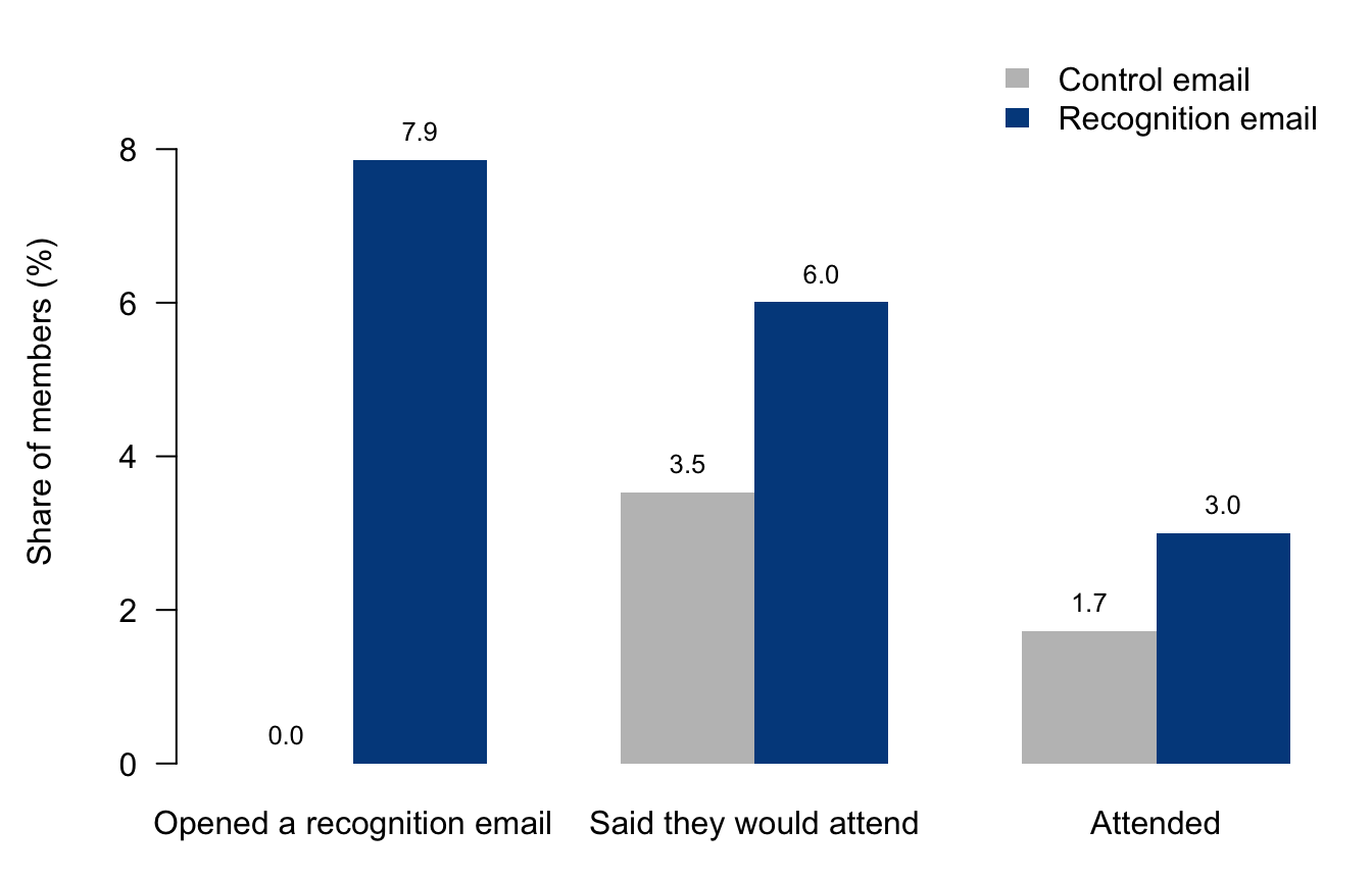
The left pair of bars shows the first stage. No one in the control group could open a recognition email, and about 8% of those sent one opened it. The other two pairs show reduced forms. In each pair, the difference between the gray and blue bars is the effect of being sent the email, not of reading it.
1.3.2 Guiso, Sapienza and Zingales (2016)
The main sample (gsz) covers cities in northern and central Italy. The instrument is whether a city was the seat of a bishop in the Middle Ages, the treatment is whether it became a free city-state, and the outcome is the number of nonprofit organizations per capita. gsz_south holds southern cities, where free city-states did not form; Chapter 5 uses it for a placebo test.
ticks <- c(0, 1, 3, 10, 30, 100, 300, 1000)
strip <- function(y, g, main) {
  stripchart(log1p(y) ~ g, vertical = TRUE, method = "jitter", jitter = 0.25,
             pch = 1, cex = 0.4, col = adjustcolor("#004a8c", 0.3), xaxt = "n", yaxt = "n",
             ylim = log1p(c(0, 1000)), main = main, cex.main = 1, font.main = 1,
             ylab = "Nonprofits per capita (log scale)")
  axis(2, at = log1p(ticks), labels = ticks, las = 1)
  axis(1, at = seq_along(levels(g)), labels = levels(g), gap.axis = -1, cex.axis = 0.9)
  med <- tapply(log1p(y), g, median)
  segments(seq_along(med) - 0.3, med, seq_along(med) + 0.3, med, lwd = 2)
}
bishop <- factor(gsz$bishopcity, labels = c("No bishop", "Bishop"))
cell <- factor(paste(gsz$bishopcity, gsz$libero_comune_allnord),
               labels = c("No bishop,\nnot free", "No bishop,\nfree",
                          "Bishop,\nnot free", "Bishop,\nfree"))
par(mfrow = c(1, 3), mar = c(4.5, 4.5, 2, 1), mgp = c(3, 1.5, 0))
share <- 100 * tapply(gsz$libero_comune_allnord, bishop, mean)
bp <- barplot(share, col = "#004a8c", border = NA, ylim = c(0, 45), las = 1,
              ylab = "Free city-states (%)", main = "(a) Treatment by instrument",
              cex.main = 1, font.main = 1)
text(bp, share, sprintf("%.1f%%\n(n = %d)", share, table(bishop)), pos = 3, cex = 0.9)
strip(gsz$totassoc_p, cell, "(b) Outcome, main sample")
strip(gsz_south$totassoc_p, factor(gsz_south$bishopcity, labels = c("No bishop", "Bishop")),
      "(c) Outcome, southern cities")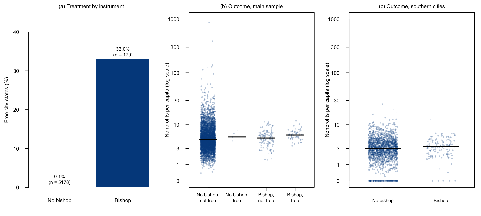
Panel (a) shows the first stage: a third of bishop seats became free city-states, compared with almost none of the other cities. Panel (b) shows the outcome for each combination of instrument and treatment; the black lines mark the medians. Only five cities are free city-states without a bishop, so nearly all the comparison runs through bishop seats. Because the outcome is very skewed, the axis uses a log scale. Panel (c) shows the same outcome in the south, by bishop seat.