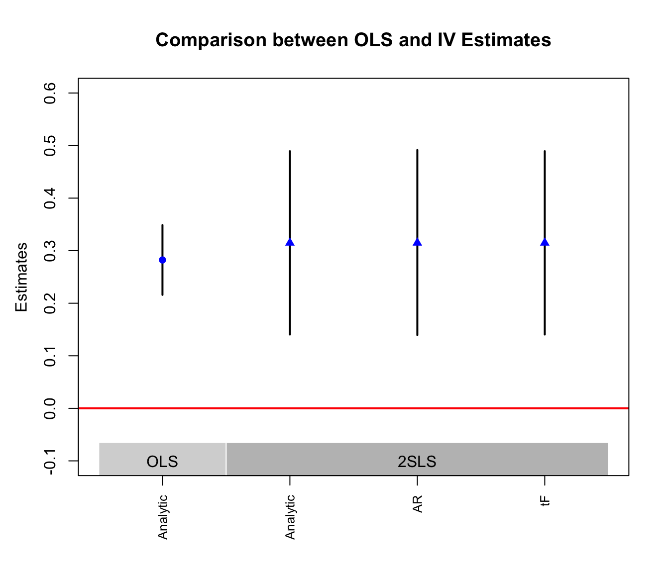
library(ivDiag)
Y <- "intended" # Y: outcome of interest
D <- "openedesteem" # D: endogenous treatment
Z <- "esteem" # Z: instrumental variable
controls <- cl <- weights <- FE <- NULL # no controls, clusters, weights or fixed effects

table(assigned = mcclendon$esteem, opened = mcclendon$openedesteem)
#>         opened
#> assigned    0    1
#>        0 1217    0
#>        1 2239  191
fs <- diff(tapply(mcclendon$openedesteem, mcclendon$esteem, mean)) # first stage
rf <- diff(tapply(mcclendon$intended, mcclendon$esteem, mean)) # reduced form
c(first_stage = unname(fs), reduced_form = unname(rf), wald_ratio = unname(rf / fs))
#>  first_stage reduced_form   wald_ratio
#> 0.07860082 0.02474952 0.314876082 Estimation and Inference
We use McClendon (2014) to illustrate estimation and inference with ivDiag. The study asks whether the promise of social esteem (being recognized by one’s peers) draws people into contentious politics. The author worked with an LGBT advocacy organization that invited its members to a Pride rally by email. Members were randomly assigned to a control email or to one of two emails that promised to recognize attendees publicly. Recognition would appear in the organization’s newsletter or on its Facebook page.
Not everyone opened the email. Random assignment to a recognition email (esteem) is therefore an instrument for opening one (openedesteem), and the 2SLS estimate is the effect of reading the promise among those who opened the email because they were sent it. Because the instrument is randomly assigned, its validity rests on the design, and its strength comes from the experiment rather than from modeling choices. Only members assigned to a recognition email could open one, so noncompliance is one-sided.
| Summary | |
|---|---|
| Unit of analysis | individual (member of the organization) |
| Treatment | opening an email that promises public recognition |
| Instrument | random assignment to such an email |
| Outcome | stated intention to attend the rally (RSVP) |
| Model | Table 2(1) |
2.1 Visualizing the first stage
With a binary instrument and a binary treatment, the first stage is a comparison of two means. Only people assigned to a recognition email could open one, and about 8% of them did. The 2SLS estimate is the ratio of the reduced form (the difference in RSVP rates) to the first stage (the difference in opening rates).
2.2 Omnibus function
The omnibus function ivDiag estimates OLS and 2SLS models and quantifies uncertainty using multiple inferential methods. It also reports first-stage F-statistics and AR test results. Members were assigned one by one, so heteroskedasticity-robust standard errors (SEs) are appropriate here. When units are assigned or sampled in groups, pass the group identifier to cl. The function then reports cluster-robust SEs and F statistics and resamples whole clusters in the bootstrap.
2.2.1 OLS estimation and inferential results
est_ols stores OLS results from the linear model lfe::felm(Y ~ D + controls | FE | 0 | cl, data = df, weights = weights). It also stores inferential results based on analytic SEs and two (block-)bootstrap methods, the coefficient method (bootstrap-c) and t-ratio method (bootstrap-t).
g$est_ols
#>            Coef     SE      t CI 2.5% CI 97.5% p.value
#> Analytic 0.2823 0.0339 8.3291  0.2159   0.3488       0
#> Boot.c   0.2823 0.0356 7.9231  0.2166   0.3547       0
#> Boot.t   0.2823 0.0339 8.3291  0.2123   0.3523       0
2.2.2 2SLS estimation and inferential results
est_2sls stores 2SLS results from lfe::felm(), along with analytic SEs and two bootstrapped SEs.
g$est_2sls
#>            Coef     SE      t CI 2.5% CI 97.5% p.value
#> Analytic 0.3149 0.0890 3.5376  0.1404   0.4893   4e-04
#> Boot.c   0.3149 0.0932 3.3798  0.1293   0.4994   2e-03
#> Boot.t   0.3149 0.0890 3.5376  0.1363   0.4934   1e-03
Two additional inferential methods are provided. AR stores results from the AR test, including the test statistic, the p-value, the 95% confidence set obtained by inverting the test (Chernozhukov and Hansen 2008), and whether the set is bounded. The set is computed exactly on the whole real line. With one instrument it is a bounded interval, the union of two unbounded rays, the whole real line, or (rarely) empty; the last three are reported with AR$bounded = FALSE. With a strong instrument, as here, it is a bounded interval close to the analytic CI.
g$AR
#> $Fstat
#>         F       df1       df2         p
#>   11.9462    1.0000 3645.0000    0.0006
#>
#> $ci.print
#> [1] "[0.1394, 0.4917]"
#>
#> $ci
#> [1] 0.1394 0.4917
#>
#> $bounded
#> [1] TRUE
tF stores results from the tF procedure based on Lee et al. (2022) as a named vector. It is returned only with one instrument. tF["cF"] is the critical value for the valid t test, adjusted based on the effective F statistic. The CI is tF["Coef"] plus or minus tF["cF"] times tF["SE"]. Lee et al. (2022) show that cF reaches 1.96 at an effective F of about 104.7. The function tF() interpolates their table and returns exactly 1.96 from F = 106.09 (10.3 squared). Below F = 4, where the table starts, tF() returns cF = Inf and a CI that covers the whole real line: the valid critical value is infinite when F is at most 3.84 and above 18.66 between 3.84 and 4.
g$tF
#>        F       cF     Coef       SE        t   CI2.5%  CI97.5%  p-value
#> 207.1798   1.9600   0.3149   0.0890   3.5376   0.1404   0.4893   0.0004
2.2.3 Characterizing the first stage
F_stat stores first-stage partial F-statistics, which assess the strength of the instruments. These include F statistics based on classic analytic SEs, robust SEs, and cluster-robust SEs (if cl is supplied). They also include the (blocked-)bootstrapped F statistic and the effective F statistic (Olea and Pflueger 2013).
g$F_stat
#>  F.standard    F.robust   F.cluster F.bootstrap F.effective
#>    103.7604    207.1798          NA    209.7429    207.1798
rho stores the Pearson correlation coefficient between the treatment and the predicted treatment from the first-stage regression, with all covariates partialled out.
g$rho
#> [1] 0.1664
est_fs stores results from the first stage regression. Both analytic and (block-)bootstrap SEs are recorded (bootstrap-c). The CIs are based on the bootstrap percentile method.
g$est_fs
#>          Coef     SE p.value   SE.b CI.b2.5% CI.b97.5% p.value.b
#> esteem 0.0786 0.0055       0 0.0054   0.0683    0.0892         0
2.2.4 Other relevant information
est_rf stores results from the reduced form regression. SEs and CIs are computed similarly to those in est_fs.
g$est_rf
#>          Coef     SE p.value   SE.b CI.b2.5% CI.b97.5% p.value.b
#> esteem 0.0247 0.0072   5e-04 0.0075   0.0106     0.039     0.002
p_iv stores the number of instruments. N and N_cl store the number of observations and the number of clusters used in the OLS and 2SLS regressions. df stores the remaining degrees of freedom from the 2SLS regression. nvalues stores the number of distinct values of the outcome Y, the treatment D, and each instrument in Z in the 2SLS regression.
g$p_iv
#> [1] 1
g$N
#> [1] 3647
g$N_cl
#> NULL
g$df
#> [1] 3645
g$nvalues
#>      intended openedesteem esteem
#> [1,]        2            2      2
To turn off bootstrapping, set bootstrap = FALSE.
ivDiag(data = mcclendon, Y = Y, D = D, Z = Z, bootstrap = FALSE)2.3 Coefficients and CIs plot
The plot_coef() function plots OLS and 2SLS estimates using different inferential methods. It also shows the effective F-statistic and the numbers of observations and clusters. The function uses base R graphics, so users can further modify the plot.
In this example, the 2SLS estimate is slightly larger than the OLS estimate. For each estimator, the CIs from the different inferential methods nearly coincide, as one would expect with a randomized, strong instrument and a large sample.
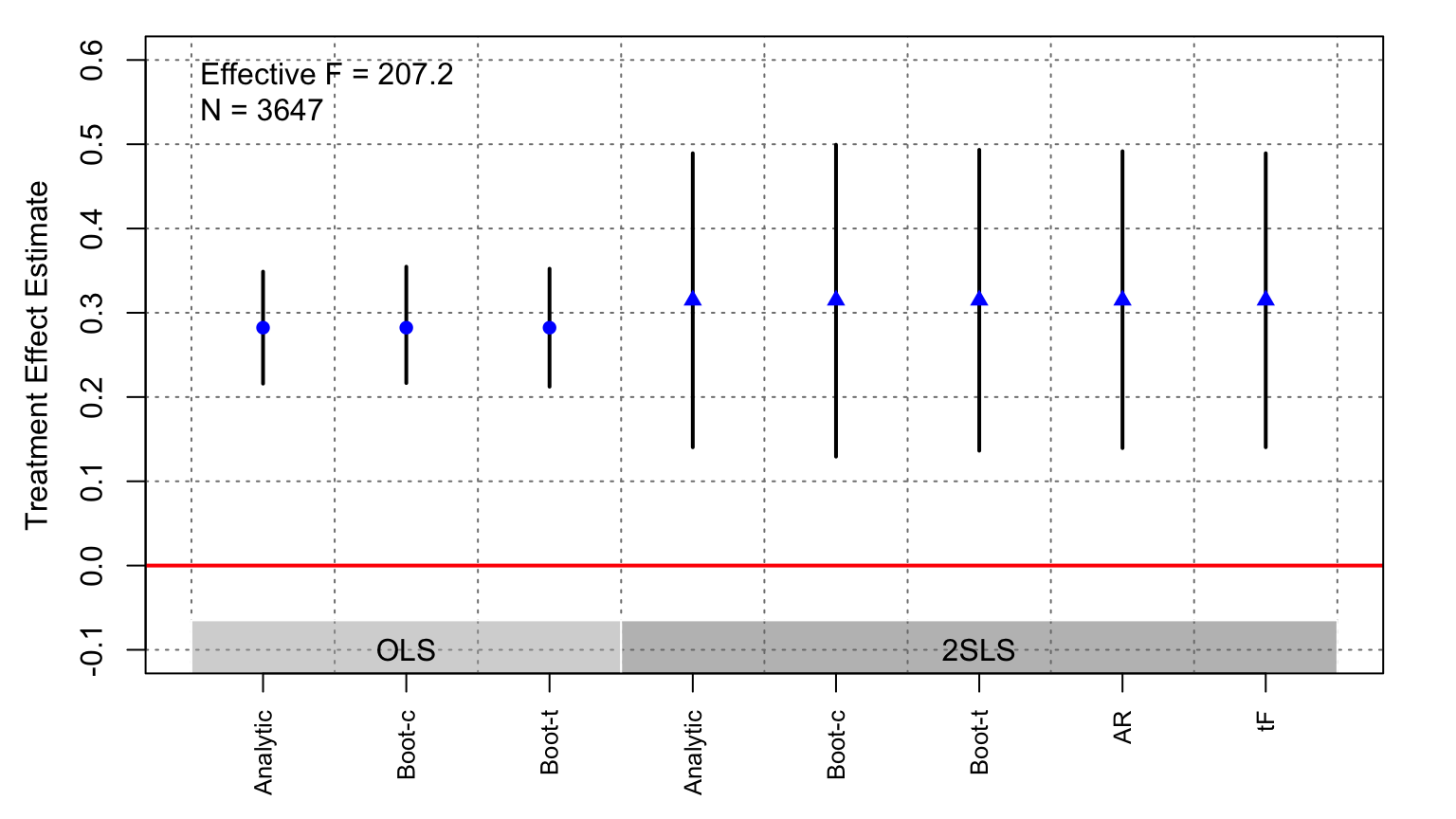
Use the plot options to adjust its appearance and select which estimates to show. For example: