library(ivDiag)
set.seed(2)
n <- 2000
x <- runif(n, -1, 1)
u <- rnorm(n)
d <- as.numeric(0.2 + 0.6 * x + 0.3 * (x >= 0) + 0.3 * u + rnorm(n, sd = 0.3) > 0.5)
y <- 2 * d + 1.5 * x - x^2 + u
p_hat <- 0.2 + 0.6 * x + 0.3 * (x >= 0)  # treatment predicted from the rule
rd <- data.frame(y = y, d = d, x = x, p_hat = p_hat)4 Fuzzy RD Designs
Some instruments come from a rule with a cutoff. A program is mandatory above a population threshold, or a polling station is added each time registered voters exceed a cap. Such a design is a fuzzy regression discontinuity (RD) design, and only the jump at the cutoff is as good as random. A treatment “predicted” from the rule also varies smoothly with the running variable, the variable behind the rule. Because this smooth variation may affect the outcome directly, it can make the first stage look much stronger than the jump alone.
To specify a fuzzy RD design in ivDiag, use running and cutoff. The instrument is the indicator for crossing the cutoff. The controls include a polynomial in the distance to the cutoff, fitted separately on each side, so that only the jump identifies the effect. Set the polynomial order with rd.poly (1 by default).
To restrict the sample to units within a given distance of the cutoff, use bandwidth. These units receive triangular kernel weights by default. For equal weights, set kernel = "uniform". Without a bandwidth, the whole sample receives equal weights, and rd$kernel reports "uniform". With several cutoffs, each unit is compared with its nearest cutoff, and cutoff fixed effects are added.
4.1 A simulated example
In the simulated example below, take-up rises smoothly with the running variable and jumps at zero. The “predicted” treatment follows both.
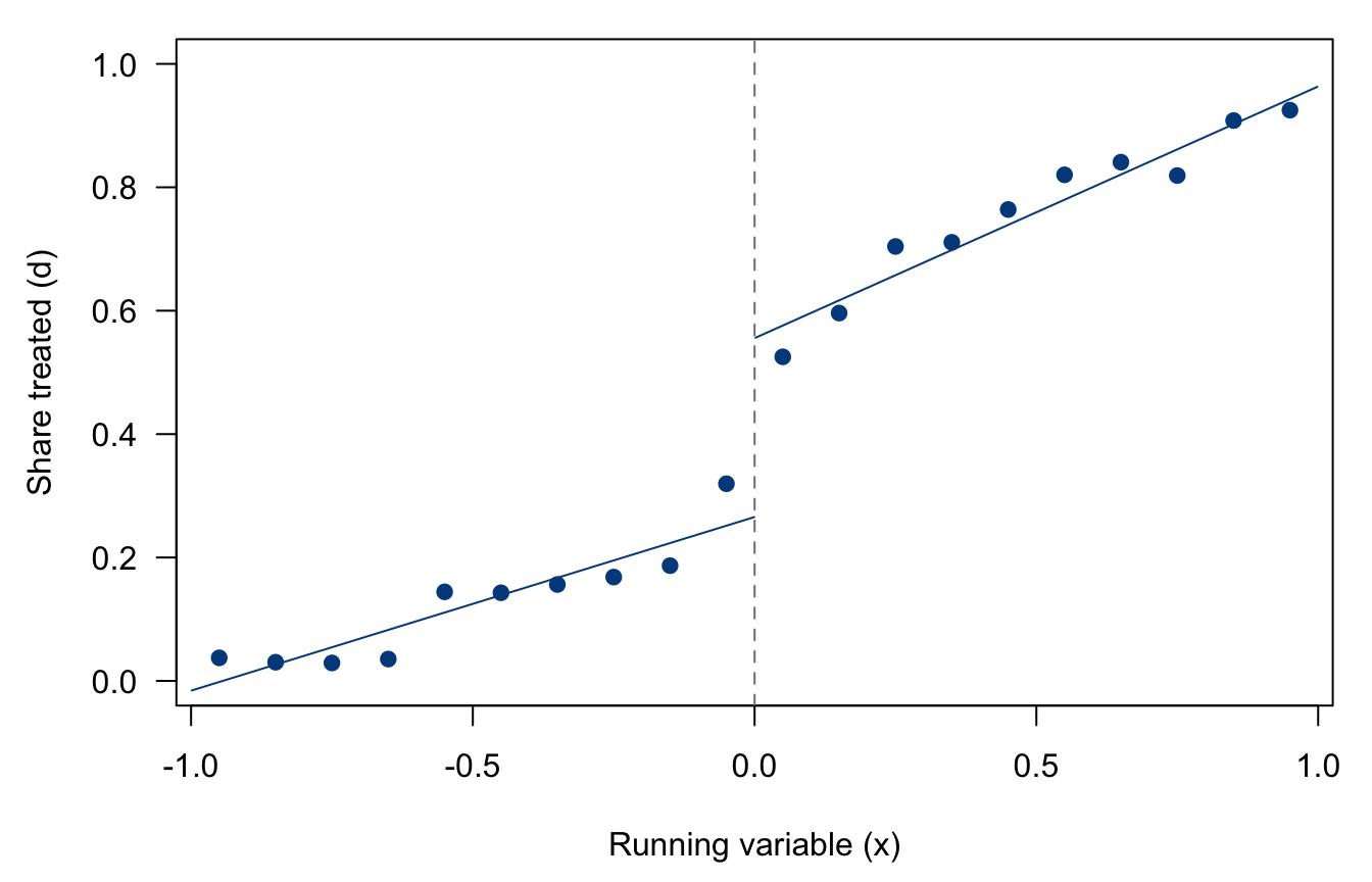
Figure 4.1 shows the share treated in narrow bins of x, with a straight line fitted on each side of the cutoff. Take-up rises with x on both sides. The gap between the two lines at zero is the jump that a fuzzy RD uses.
bins <- cut(x, seq(-1, 1, by = 0.1))
mid <- seq(-0.95, 0.95, by = 0.1)
par(mar = c(4.5, 4.5, 1, 1))
plot(mid, tapply(d, bins, mean), pch = 19, col = "#004a8c", ylim = c(0, 1),
     xlab = "Running variable (x)", ylab = "Share treated (d)", las = 1)
abline(v = 0, lty = 2, col = "gray50")
for (side in list(x < 0, x >= 0)) {
  fit <- lm(d ~ x, subset = side)
  xs <- range(x[side])
  lines(xs, predict(fit, data.frame(x = xs)), col = "#004a8c")
}
We estimate the effect twice: with the predicted treatment as the instrument, and as a fuzzy RD.
# predicted treatment as the instrument, running variable ignored
g0 <- ivDiag(data = rd, Y = "y", D = "d", Z = "p_hat", bootstrap = FALSE)
# fuzzy RD: crossing the cutoff, linear in x on each side
g1 <- ivDiag(data = rd, Y = "y", D = "d", running = "x", cutoff = 0,
             bootstrap = FALSE)
rbind(predicted = c(g0$est_2sls[1, 1:2], F.effective = g0$F_stat[["F.effective"]]),
      fuzzy_RD = c(g1$est_2sls[1, 1:2], F.effective = g1$F_stat[["F.effective"]]))
#>             Coef     SE F.effective
#> predicted 4.5637 0.0736   2378.0964
#> fuzzy_RD  1.5637 0.3391     54.9075
g1$rd
#> $running
#> [1] "x"
#>
#> $cutoff
#> [1] 0
#>
#> $poly
#> [1] 1
#>
#> $bandwidth
#> NULL
#>
#> $kernel
#> [1] "uniform"
#>
#> $N_left
#> [1] 1002
#>
#> $N_right
#> [1] 998
The predicted-treatment instrument reports a far stronger first stage and a biased estimate (the true effect is 2). This occurs because it also uses the smooth relationship between x and both d and y. The fuzzy RD uses only the jump at the cutoff. Its instrument is weaker but valid, and its AR set and the tF procedure account for that weakness (Feir et al. 2016).
4.2 Polling station size and vote buying
Rueda (2017) asks whether smaller polling stations make vote buying easier to enforce in Colombia, since brokers can check the published results of small groups of voters. By law, a polling station may serve at most a fixed number of registered voters: 400 in 2006 and 2007, 500 in 2010, and 350 in 2011. Each time a municipality’s registered voters cross a multiple of this cap, one more station opens. The rule therefore predicts a drop in the average station size. The study uses the predicted size as the instrument for the actual size.
| Summary | |
|---|---|
| Unit of analysis | municipality in one election |
| Treatment | average polling station size, in logs (lm_pob_mesa) |
| Instrument | average size predicted by the rule, in logs (lz_pob_mesa_f) |
| Outcome | incidence of vote buying (e_vote_buying) |
| Controls | log population, log registered voters |
The rueda data do not record the election year, so we recover the cap. Most municipalities appear in all four elections, and their rows are in election order, so the row gives the year and the cap. The rule confirms this order: in every row where only one cap reproduces the predicted size (registered voters divided by the number of stations the rule requires), that cap is the one for the row’s year. For the other municipalities, we take the cap whose rule reproduces the predicted size. We then measure registered voters in units of the cap (ratio). A new station opens each time ratio crosses an integer, so every integer is a cutoff.
voters <- exp(rueda$lpotencial)  # registered voters
caps <- c(350, 400, 500)
err <- sapply(caps, function(cap) abs(log(voters / ceiling(voters / cap)) - rueda$lz_pob_mesa_f))
cap_rule <- caps[apply(err, 1, which.min)]  # the cap whose rule reproduces the predicted size
# municipalities in all four elections: rows are in election order (2006, 2007, 2010, 2011)
pos <- ave(seq_along(voters), rueda$muni_code, FUN = seq_along)
n_obs <- ave(seq_along(voters), rueda$muni_code, FUN = length)
rueda$cap <- ifelse(n_obs == 4, c(400, 400, 500, 350)[pos], cap_rule)
rueda$ratio <- voters / rueda$cap
table(rueda$cap)
#>
#>  350  400  500
#> 1101 2157 1094
quantile(rueda$ratio, c(0.1, 0.5, 0.9))
#>       10%       50%       90%
#>  7.230751 20.229464 84.006892
Figure 4.2 plots each municipality-election with ratio below 10.5 (no municipality has fewer than 1.4 times the cap). The vertical axis shows the actual average station size as a share of the cap, and the line shows the size predicted by the rule. Between two cutoffs, the predicted size rises steadily with registered voters. At each cutoff, it drops. These drops shrink as ratio grows: crossing 2, the predicted size falls from the cap to 2/3 of it, but crossing 10, only to 10/11 of it. Many municipalities have one or two more stations than the rule requires, forming lower copies of the saw-tooth pattern, so their size does not follow the rule’s drops.
near <- subset(rueda, ratio < 10.5)
grid <- seq(1.3, 10.5, by = 0.001)
par(mar = c(4.5, 4.5, 2.5, 1))
plot(near$ratio, exp(near$lm_pob_mesa) / near$cap, pch = 1, cex = 0.5,
     col = adjustcolor("#004a8c", 0.5), xlim = c(1.3, 10.5), las = 1,
     xlab = "Registered voters / cap", ylab = "Average station size / cap")
lines(grid, grid / ceiling(grid), col = "gray30")
legend("top", inset = c(0, -0.1), xpd = TRUE, horiz = TRUE, bty = "n",
       legend = c("Municipality-election", "Predicted by the rule"),
       pch = c(1, NA), lty = c(NA, 1), col = c("#004a8c", "gray30"))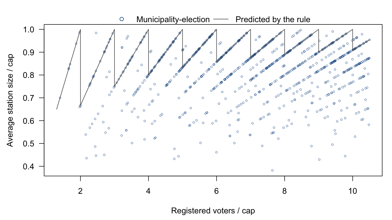
To specify the fuzzy RD, pass the running variable and the integers as cutoffs. ivDiag then compares each municipality with its nearest cutoff and adds cutoff fixed effects. The size of the drop differs by cutoff: crossing k lowers the log predicted size by log((k + 1)/k), which is 0.41 at 2 but 0.05 at 20. An indicator for crossing would impose the same drop at every cutoff. We therefore take the log of ratio as the running variable and the logs of the integers as cutoffs, and pass the predicted size as Z. With registered voters among the controls, the polynomial by side and the cutoff fixed effects, the only variation left in the predicted size is the drop at each cutoff, at the size the rule gives it. Below, we fit the first stage four ways and report only the first-stage F statistics.
ctrl <- c("lpopulation", "lpotencial")
# predicted size as the instrument, running variable ignored
f_pred <- ivDiag(data = rueda, Y = "e_vote_buying", D = "lm_pob_mesa",
                 Z = "lz_pob_mesa_f", controls = ctrl, cl = "muni_code",
                 bootstrap = FALSE, run.AR = FALSE)
# the same, with fixed effects for the cap (one cap per election year)
f_cap <- ivDiag(data = rueda, Y = "e_vote_buying", D = "lm_pob_mesa",
                Z = "lz_pob_mesa_f", controls = ctrl, FE = "cap", cl = "muni_code",
                bootstrap = FALSE, run.AR = FALSE)
# fuzzy RD: the drops at the cutoffs, each as large as the rule makes it
rueda$lratio <- log(rueda$ratio)
f_rd <- ivDiag(data = rueda, Y = "e_vote_buying", D = "lm_pob_mesa",
               Z = "lz_pob_mesa_f", controls = ctrl, cl = "muni_code",
               running = "lratio", cutoff = log(1:ceiling(max(rueda$ratio))),
               bootstrap = FALSE, run.AR = FALSE)
# the same, below the tenth cutoff
f_rd10 <- ivDiag(data = subset(rueda, ratio < 10.5), Y = "e_vote_buying",
                 D = "lm_pob_mesa", Z = "lz_pob_mesa_f", controls = ctrl,
                 cl = "muni_code", running = "lratio", cutoff = log(1:11),
                 bootstrap = FALSE, run.AR = FALSE)
rbind(predicted = f_pred$F_stat, predicted_cap_FE = f_cap$F_stat,
      fuzzy_RD = f_rd$F_stat, fuzzy_RD_below_10 = f_rd10$F_stat)
#>                   F.standard  F.robust F.cluster F.effective
#> predicted          3106.3869 3108.5914 8598.3264   8598.3264
#> predicted_cap_FE     44.4654   28.5878   16.4999     16.4999
#> fuzzy_RD              3.2385    1.9175    1.6629      1.6629
#> fuzzy_RD_below_10     4.6463    4.4094    3.9545      3.9545
With the predicted size as the instrument, the effective F statistic is 8,598. Little of this strength comes from the drops at the cutoffs. Registered voters are a control, so the steady rise between cutoffs is partialled out. Most of what remains is the change in the cap across elections, from 400 to 500 to 350, which shifted the predicted size of every station at once. With fixed effects for the cap, the effective F statistic falls to 16.5. In the fuzzy RD, only the drops at the cutoffs identify the effect, and the effective F statistic is 1.66. Below the tenth cutoff, where the drops are largest, it is 3.95.
The drops are weak in the data because few municipalities have the number of stations the rule requires.
stations <- round(voters / exp(rueda$lm_pob_mesa))  # stations in each municipality-election
required <- ceiling(rueda$ratio)                     # stations the rule requires
round(c(exact = mean(stations == required), more = mean(stations > required)), 2)
#> exact  more
#>  0.16  0.79
round(tapply(stations == required, cut(rueda$ratio, c(0, 5.5, 20.5, Inf)), mean), 2)
#>    (0,5.5] (5.5,20.5] (20.5,Inf]
#>       0.52       0.24       0.05
Only 16% of municipality-elections have exactly the required number, and 79% have more. The share falls as municipalities grow, and half of them have more than 20 times the cap, where crossing a cutoff lowers the predicted size by less than 5%. With a first stage this weak, rely on the AR set rather than the t-test (Feir et al. 2016).