Interflex with DML Estimators • interflex

Installation

To use double/debiased machine learning (DML) estimators, please install the interflex package diretly from Github:

devtools::install_github('xuyiqing/interflex')

Set up Python environment

To use DML estimators in interflex, we rely on several Python packages. The integration between R and Python is facilitated by the reticulate package, which allows R to interface with Python seamlessly. The following steps set up a Python environment with all required dependencies.

First, install the reticulate package in R. This package enables R to interface with Python.

install.packages("reticulate", repos = 'http://cran.us.r-project.org', force = TRUE)

Then, we use Miniconda, a minimal installer for Conda. Miniconda helps manage Python environments and packages. By default, the installation process will create a virtual environment named r-reticulate.

reticulate::install_miniconda(update = TRUE)

With Miniconda installed, we point to the platform using use_condaenv. This step is incorporated in the interflex package.

reticulate::use_condaenv(condaenv = "r-reticulate")

Finally, install the necessary Python libraries. These libraries include tools for statistical modeling and machine learning that are essential for using the interflex package.

reticulate::py_install(packages = c("patsy", "numpy", "pandas",
                                    "scikit-learn", "doubleml", "econml"))

Some Mac users may encounter a “*** caught segfault ***” error. In that case, we recommend setting up a virtual environment. In Terminal, type:

python3 -m venv ~/.virtualenvs/myenv
source ~/.virtualenvs/myenv/bin/activate

Then install all Python packages there:

pip install numpy
pip install patsy
pip install pandas
pip install scikit-learn
pip install econml
pip install doubleml

In R, point to the newly set up environment myenv:

reticulate::use_virtualenv("myenv")

Load packages

These are packages are necessary for this tutorial:

library(interflex)
library(ggplot2)
library(ggpubr)
library(rmarkdown)
library(patchwork)

reticulate::use_virtualenv("myenv") ## point to your Python environment

This vignette gives a brief overview of estimating conditional marginal effects (CME) using the interflex pacakge, focusing on the Double/debiased Machine Learning (DML) estimator. This vignette walks through using DML estimators for different empirical setup, using both the simulating data and real-world data, including:

DML Estimators

Binary treatment with discrete outcomes
Continuous treatment with discrete outcome

Applications

Application 1: Binary Treatment with Continuous Outcomes
Application 2: Continuous Treatment with Continuous Outcomes

Overview of Methodology

This section explores the basic ideas behind the DML framework, which enables the use of modern machine learning techniques to robustly estimate CME. The DML estimators for CME is first developed in Semenova and Chernozhukov (2021), and is expanded by Bonvini et al. (2023).

Estimand

We begin by formally defining CME using the Neyman–Rubin potential outcome framework Rubin (1974). Let $Y_i(d)$ be the potential outcomes corresponding to a unit $i$ ’s response to potential treatment value $D_i = d$ . $X_i$ are the moderator of interest, along with $Z_i$ be the vector of covariates. We can define the full set of covariates as $V_i = (X_i, Z_i)$ . The CME of treatment $D$ on $Y$ by $X$ is:

$\theta(x) = \mathbb{E}\left[\frac{\partial Y_i(d)}{\partial D} \mid X_i = x \right]$

When $D_{i}$ is binary, it simplifies to $\mathbb{E}[Y_i(1) - Y_i(0) \mid X_i = x]$ , which is essentially Conditional Average Treatment Effect (CATE) at covariate value $v$ , $\tau(v) = \mathbb{E}[Y_i(1) - Y_i(0) \mid V_i = v]$ , marginalized over the distribution of additional covariates $Z_{i}$ .

Note that the defintion has implied the stable unit treatment value assumption (SUTVA):

SUTVA: $Y_i(d_{1}, d_{2}, \cdots, d_{n}) = Y_i(d_{i})$ . For each unit $i$ , there is only one potential outcome $Y_i(d_i)$ for each possible treatment they could receive.

Idenfitication assumptions

In the cross-sectional setting, we assume STUVA, unconfoundedness and strict overlap.

Unconfoundedness: $\{ Y_i(d_{i}) \} \perp\!\!\!\perp D_i \mid V_i = v, \text{ for all } v \in \mathscr{V}$ . Potential outcome $Y_i(d_{i}$ are independent of the treatment $D_i$ , conditioning on covariates $V_i = v$ .
Strict overlap: $f_{D \mid V}(d \mid v) > 0$ for all $d \in \mathscr{D}$ and $v \in \mathscr{V}$ , where $\mathscr{D}$ is the support of the treatment $D$ , $\mathscr{V}$ is the support of the covariates $V$ , and $f_{D \mid V}(d \mid v)$ is the conditional probability density function of $D$ given $V$ .

When $D$ is binary, it simplifies to: For some positive $\eta$ , $\eta \leq \mathbb{P}(W_i = 1 \mid V_i = v) \leq 1-\eta,\quad\text{with probability } 1.$ This assumption states that every unit $i$ must have a non-zero probability of being assigned to each treatment condition.

The DML framework

When $D$ , $X$ and $Z$ are all discrete, we can estimate $\mathbb{E}[Y(1)-Y(0)|X]$ nonparametrically. However, when one of them is continuous or high-dimensional, CME becomes difficult to estimate without imposing functional form assumptions. These assumptions can be too restrictive and easily violated in practice.

Here, we introduce the double/debiased machine learning (DML) estimator, to flexibly estimate CME under mild conditions. The primary advantage of DML lies in its ability to use machine learning method to estimate nuisance parameters $\eta_0$ (parameters that are not of direct interest to researchers), in nonparametric, data-driven way, while providing valid inference for the target quantity, in this case, the CME $\theta_0$ .

Building on the principles of doubly robust estimation, DML is introduced by Chernozhukov et al. (2018) to estimate low-dimensional parameter $\theta_0$ in the presence of high-dimensional nuisance parameter $eta_0$ . DML extends the doubly robust framework by integrating machine learning algorithms to flexibly model both the outcome and the treatment assignment processes.

The DML method yields unbiased, $\sqrt{n}$ -consistent estimators and confidence intervals for the low-dimensional parameter of interest, $\theta_0$ , even in the presence of potentially high-dimensional nuisance parameters $\eta_0$ . Crucially, it achieves this without imposing stringent assumptions on high-dimensional covariates, instead deriving these forms directly from the data.

The three key ingredients of the DML framework are:

Neyman orthogonality, which ensures the bias in estimating $\eta_0$ doesn’t spillover to $\theta_0$ ;
High-quality ML method, to ensure the estimated nuisance parameter $\hat{\eta}$ converges to the true parameter at a fast enough rate;
Cross-fitting, to help mitigate overfitting biases.

If these three assumptions are met, i.e., that (1) the Neyman-orthogonal score is constructed for the parameter of interest $\theta_0$ , and (2) the nuisance functions are estimated with enough accuracy and are cross fitted, the DML estimator achieves the $\sqrt{n}-$ rate of convergence and is approximately normally distributed. Both the rate of concentration and the distributional approximation holds uniformly over a broad class of probability distributions.

Model

In the interflex pacakge, for CME with binary treatment, the data-generating process (DGP) is modeled through Interactive Regression Model (IRM); For CME with continuous treatment, the DGP is modeled through Partially Linear Regression Model (PLR).

In practice with binary treatment, the IMR has the form:

$Y =g(V, D) + \epsilon,\ E[\epsilon \mid V, D] = 0$ $D = m(V) + \eta, \ E[\eta \mid V] = 0$

With continuous treatment, the PLR has the form: $Y = \theta(V)D + g(V) + \epsilon,\ E[\epsilon \mid V, D] = 0$ $D = m(V) + \eta, \ E[\eta \mid V] = 0$

where:

$g(\cdot)$ is a nonparametric function capturing the relationship between full set of covaraites $V_i = (X_i, Z_i)$ and the outcome $Y$ .
$m(\cdot)$ is a nonparametric function capturing the relationship between full set of covaraites $V_i = (X_i, Z_i)$ and the treatment $D$ (when $D$ is binary, it is also the propensity score function).
$\epsilon,\eta$ are disturbances.

Note that when $D$ is binary, $Y =g(V, D) + \epsilon$ can be written as $Y = \theta(V)D + g(V) + \epsilon$ without loss of generality.

Procedure

The DML framework for CME operates through the following steps:

1. Estimate nuisance functions

Outcome model: Estimate the nuisance function $g(\cdot)$ using ML methods.
Treatment model: Estimate the nuisance function $m(\cdot)$ using ML methods.

2. Apply the Neyman orthogonality condition

The key of DML is the construction of orthogonal score to meet the Neyman orthogonality condition.

In IRM, the orthogonal signal $\Lambda(\eta)$ is constructed through AIPW correction to meet the form:

$\Lambda(\eta) = \mu(1, V) - \mu(0, V) + \frac{D(Y - \mu(1, V))}{e(V)} - \frac{(1 - D)(Y - \mu(0, V))}{1 - e(V)}$

In PLR, the orthogonal signal is constructed via “partialling out” to meet the form:

$\Lambda(\eta) = -\partial_d \log e(d\mid v)\,[Y-\mu(d,v)] + \partial_d\mu(d,v)$

3. Dimension reduction

The constructed orthogonal signal is projected onto a functional space in $X$ , which, in the interflex package, is either a B-spline or kernel regression, to recover CME $\theta(x)$ .

DML Estimators

Load the simulated toy datasets, s6, s7, and s9, for this tutorial. s6 is a case of a binary treatment indicator with discrete outcomes. s7 is a case of a continuous treatment indicator with discrete outcomes. s9 is a case of a discrete treatment indicator (3 groups) with discrete outcomes.

data(interflex)
ls()
#>  [1] "app_hma2015"    "app_vernby2013" "s1"             "s2"            
#>  [5] "s3"             "s4"             "s5"             "s6"            
#>  [9] "s7"             "s8"             "s9"

When setting the option estimator to DML, the function will conduct the two-stage DML estimator to compute the marginal effects. In the following command, the outcome variable is “Y”, the moderator is “X”, the covariates are “Z1” and “Z2”, and here it uses logit link function. ml_method determines the machine learning model used in estimating nuisance function, treat.type set the data type of treatment variable, it can be either continuous or discrete. Here, we use dataset s6,as an example. Since s6 binary treatment indicator with discrete outcomes, we set treat.type to discrete.

Binary treatment with discrete outcomes

To implement the DML estimator, we need to set the option estimator='DML' and specify two machine learning models: one for the outcome model (via the option model.y) and one for the treatment model (via the option model.t). Here, we use a neural network model (nn) for the outcome model and a random forest model (rf) for the treatment model. The gray area depicts the pointwise interval, while the dashed line marks the uniform/joint confidence interval.

s6.DML.nn.rf <- interflex(estimator="DML", data = s6,
                                 Y = "Y", D = "D", X = "X", Z = c("Z1", "Z2"),
                                 model.y = "nn",model.t = "rf")
#> Baseline group not specified; choose treat = 0 as the baseline group.
plot(s6.DML.nn.rf)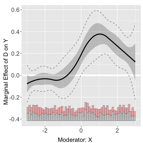

The estimated treatment effects of $D$ on $Y$ across the support of $X$ are saved in:

## printing the first 10 rows
lapply(s6.DML.nn.rf$est.dml, head, 10)
#> $`1`
#>            X          ME         sd lower CI(95%) upper CI(95%)
#> 1  -2.998668 -0.09360447 0.05068617   -0.19294754  0.0057386046
#> 2  -2.876374 -0.08165094 0.03952928   -0.15912691 -0.0041749658
#> 3  -2.754080 -0.07085490 0.03180335   -0.13318832 -0.0085214866
#> 4  -2.631786 -0.06121637 0.02768394   -0.11547589 -0.0069568496
#> 5  -2.509492 -0.05273533 0.02654028   -0.10475332 -0.0007173434
#> 6  -2.387197 -0.04541179 0.02699490   -0.09832083  0.0074972427
#> 7  -2.264903 -0.03924575 0.02773199   -0.09359946  0.0151079487
#> 8  -2.142609 -0.03423721 0.02795324   -0.08902455  0.0205501294
#> 9  -2.020315 -0.03038617 0.02734961   -0.08399041  0.0232180782
#> 10 -1.898021 -0.02769262 0.02603008   -0.07871064  0.0233253999
#>    lower uniform CI(95%) upper uniform CI(95%)
#> 1             -0.3024237            0.11521477
#> 2             -0.2445055            0.08120364
#> 3             -0.2018798            0.06017000
#> 4             -0.1752699            0.05283720
#> 5             -0.1620772            0.05660654
#> 6             -0.1566266            0.06580306
#> 7             -0.1534973            0.07500579
#> 8             -0.1494003            0.08092584
#> 9             -0.1430623            0.08229001
#> 10            -0.1349326            0.07954731

Users can then use the plot command to visualize the treatment effects. For comparison, we can add the “true” treatment effects to the plot.

x <- s6$X
TE <- exp(-1+1+x+1*x)/(1+exp(-1+1+x+1*x))-exp(-1+0+x+0*x)/(1+exp(-1+0+x+0*x))
plot.s6 <- plot(s6.DML.nn.rf, show.all = TRUE, Xdistr = 'none')$`1`
plot.s6 + geom_line(aes(x=x,y=TE),color='red')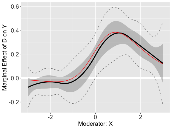

First Stage DML Model Selections

The DML estimator supports three different machine learning algorithms: rf (Random Forest), nn (Neural Network), and hgb (Histogram-based Gradient Boosting). Users can change the model.y and model.t option to calculate the nuisance parameter using a different ML method. In this example, we use the dataset s9 to demonstrate the process:

## true treatment effects
x <- s9$X
TE1 <- exp(1+x)/(1+exp(1+x))-exp(-x)/(1+exp(-x))
TE2 <- exp(4-x*x-x)/(1+exp(4-x*x-x))-exp(-x)/(1+exp(-x))

## neural network + neural network
s9.DML.nn.nn <- interflex(estimator="DML", data = s9,
                          Y = "Y", D = "D", X = "X", Z = c("Z1", "Z2"),
                          model.y = "nn",model.t = "nn")
#> Baseline group not specified; choose treat = 0 as the baseline group.

plot.s9.nn.nn.1<-plot(s9.DML.nn.nn, show.all = T)[[1]]
plot.s9.nn.nn.2<-plot(s9.DML.nn.nn, show.all = T)[[2]]
p1.nn.nn<-plot.s9.nn.nn.1 + geom_line(aes(x=x,y=TE1),color='red')
p2.nn.nn<-plot.s9.nn.nn.2 + geom_line(aes(x=x,y=TE2),color='red')


## random forest + random forest
s9.DML.rf.rf <- interflex(estimator="DML", data = s9,
                          Y = "Y", D = "D", X = "X", Z = c("Z1", "Z2"),
                          model.y = "rf",model.t = "rf")
#> Baseline group not specified; choose treat = 0 as the baseline group.

plot.s9.rf.rf.1<-plot(s9.DML.rf.rf, show.all = T)[[1]]
plot.s9.rf.rf.2<-plot(s9.DML.rf.rf, show.all = T)[[2]]
p1.rf.rf<-plot.s9.rf.rf.1 + geom_line(aes(x=x,y=TE1),color='red')
p2.rf.rf<-plot.s9.rf.rf.2 + geom_line(aes(x=x,y=TE2),color='red')


## hist gradient boosting + hist gradient boosting
s9.DML.hgb.hgb <- interflex(estimator="DML", data = s9,
                          Y = "Y", D = "D", X = "X", Z = c("Z1", "Z2"),
                          model.y = "hgb",model.t = "hgb")
#> Baseline group not specified; choose treat = 0 as the baseline group.

plot.s9.hgb.hgb.1<-plot(s9.DML.hgb.hgb, show.all = T)[[1]]
plot.s9.hgb.hgb.2<-plot(s9.DML.hgb.hgb, show.all = T)[[2]]
p1.hgb.hgb<-plot.s9.hgb.hgb.1 + geom_line(aes(x=x,y=TE1),color='red')
p2.hgb.hgb<-plot.s9.hgb.hgb.2 + geom_line(aes(x=x,y=TE2),color='red')

p1<-ggarrange(p1.nn.nn, p2.nn.nn)
p1<-annotate_figure(p1, 
                    top = text_grob("Neural Network",
                    face = "bold", size = 13))

p2<-ggarrange(p1.rf.rf, p2.rf.rf)
p2<-annotate_figure(p2,
                    top = text_grob("Random Forest",
                    face = "bold", size = 13))

p3<-ggarrange(p1.hgb.hgb, p2.hgb.hgb)
p3<-annotate_figure(p3,
                    top = text_grob("Hist Gradient Boosting",
                    face = "bold", size = 13))
 
ggarrange(p1,p2,p3, ncol = 1)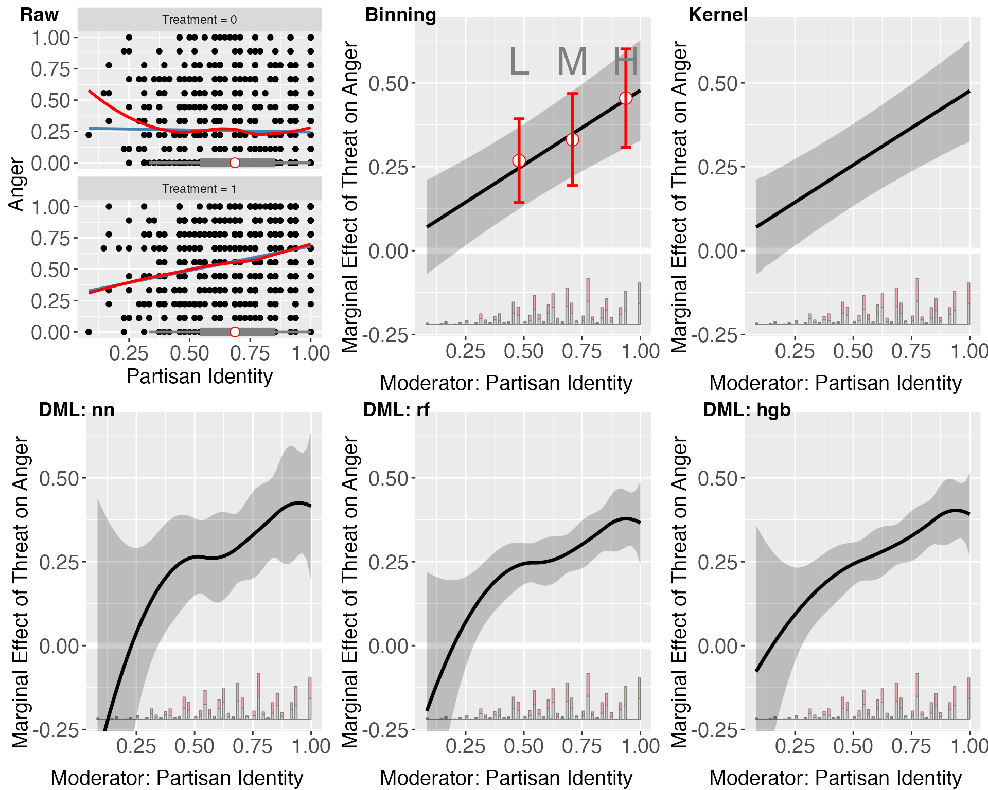

We find that different ML models give very similar results, which is expected since there are only two confounders, $Z_{1}$ and $Z_{2}$ , in the dataset, and all methods can accurately partial out their impacts on the outcome and the treatment.

Specifying Model Parameters

Continuous treatment with discrete outcome

Users can customize parameters for the machine learning model in both stages by specifying the options param.y and param.t. For the whole list of parameters that are applicable to the neural network model, users can refer to the MLPRegressor or the MLPClassifier. For the random forest method, users can refer to the RandomForestRegressor or the RandomForestClassifier. For the hist gradient boosting method, users can refer to the HistGradientBoostingRegressor or the HistGradientBoostingClassifier. Here we use dataset s7 to explore how selecting different DML parameters affects performance. We can directly specify the size of the neural networks, the activation function, learning rate, and solver using the list param_nn and feed them to the DML estimator.

param_nn <- list(
  hidden_layer_sizes = list(10L,20L,10L),
  activation = c("tanh"),
  solver = c("sgd"),
  alpha = c(0.05),
  learning_rate = c("adaptive")
)

s7.DML.nn.linear.para <- interflex(estimator="DML", data = s7,
                                       Y = "Y", D = "D", X = "X", 
                                       Z = c("Z1", "Z2"),
                                       model.y = "nn", param.y = param_nn,
                                       model.t = "nn", param.t = param_nn)

n <- nrow(s7)
d2 <- s7$D
x_values <- sort(s7$X) 
d2_value <- median(d2)  # Example value for d2

marginal_effect <- function(D_value, X_value) {
  link_value <- -1 + D_value + X_value + D_value * X_value
  prob_value <- exp(link_value) / (1 + exp(link_value))
  marginal_effect_value <- prob_value * (1 - prob_value) * (1 + X_value)
  return(marginal_effect_value)
}

# Applying the function to the range of x values to calculate true ME
ME <- sapply(x_values, function(x_val) marginal_effect(d2_value, x_val))


p.s7.nn.linear <- plot(s7.DML.nn.linear.para, show.all = TRUE, ylim = c(-0.5,0.5))[[1]]
p.s7.nn.linear<-p.s7.nn.linear + ylim(-0.5,0.5) + 
  geom_line(aes(x=x_values,y=ME),color='red')+
  ggtitle("Neural Network with Specified Parameters")+
  theme(plot.title = element_text(size=10))
#> Scale for y is already present.
#> Adding another scale for y, which will replace the existing scale.

Cross-Validation

Users can also specify the grids of parameters using the options param.grid.y and param.grid.t. The DML estimator will then search through all sequences of parameter settings and pick the most suitable one using cross-validation. We need to set the options CV to TRUE to invoke the cross-validation. As an example, we specify the grids used for the neural network, random forest, and hist gradient boosting, then we compare their performances on s7.

param_grid_nn <- list(
  hidden_layer_sizes = list(list(10L,20L,10L), list(20L)),
  activation = c("tanh","relu"),
  solver = c("sgd","adam"),
  alpha = c(0.0001,0.05),
  learning_rate = c("constant","adaptive")
)

param_grid_rf <- list(
  max_depth = c(2L,3L,5L,7L),
  n_estimators = c(10L, 30L, 50L, 100L, 200L, 400L, 600L, 800L, 1000L),
  max_features = c(1L,2L)
)

param_grid_hgb <- list(
  max_leaf_nodes = c(5L,10L,20L,30L),
  min_samples_leaf = c(5L,10L,20L),
  l2_regularization = c(0,0.1,0.5),
  max_features = c(0.5,1)
)


# nn (cv) + rf (cv) + linear
s7.cvnn.cvrf <- interflex(estimator="DML", data = s7,
                                     Y = "Y", D = "D", X = "X", Z = c("Z1", "Z2"),CV = TRUE,
                                     model.y = "nn",param.grid.y = param_grid_nn,
                                     model.t = "rf",param.grid.t = param_grid_rf)

# nn (cv) + hgb (cv) + regularization (cv)
s7.cvnn.cvhgb <- interflex(estimator="DML", data = s7,
                                     Y = "Y", D = "D", X = "X", Z = c("Z1", "Z2"),CV = TRUE,
                                     model.y = "nn",param.grid.y = param_grid_nn,
                                     model.t = "hgb",param.grid.t = param_grid_hgb)

# rf (cv) + rf (cv) + rf (cv)
s7.cvrf.cvrf <- interflex(estimator="DML", data = s7,
                                     Y = "Y", D = "D", X = "X", Z = c("Z1", "Z2"),CV = TRUE,
                                     model.y = "rf",param.grid.y = param_grid_rf,
                                     model.t = "rf",param.grid.t = param_grid_rf)

# hgb (cv) + hgb (cv) + hgb (cv)
s7.cvhgb.cvhgb <- interflex(estimator="DML", data = s7,
                                     Y = "Y", D = "D", X = "X", Z = c("Z1", "Z2"),CV = TRUE,
                                     model.y = "hgb",param.grid.y = param_grid_hgb,
                                     model.t = "hgb",param.grid.t = param_grid_hgb)

p.1<-plot(s7.cvnn.cvrf, show.all = TRUE, ylim = c(-0.5,0.9))[[1]]
p.2<-plot(s7.cvnn.cvhgb, show.all = TRUE, ylim = c(-0.5,0.9))[[1]]
p.3<-plot(s7.cvrf.cvrf, show.all = TRUE, ylim = c(-0.5,0.9))[[1]]
p.4<-plot(s7.cvhgb.cvhgb, show.all = TRUE, ylim = c(-1.5,1.5))[[1]]

## adding true treatment effects when d = 0.53 (50%) to the plots 
p.1<-p.1 + ylim(-0.5,0.9) +
  geom_line(aes(x=x_values,y=ME),color='red')+
  ggtitle("Neural Network (cv) + Random Forest (cv) + Linear")+
  theme(plot.title = element_text(size=10))

  
p.2<-p.2 +ylim(-0.5,0.9)+
  geom_line(aes(x=x_values,y=ME),color='red')+
  ggtitle("Neural Network (cv) + Random Forest (cv) + Lasso (CV)")+
  theme(plot.title = element_text(size=10))


p.3<-p.3  +ylim(-0.5,0.9)+
  geom_line(aes(x=x_values,y=ME),color='red')+
  ggtitle("Random Forest (cv) + Random Forest (cv) + Random Forest (cv)")+
  theme(plot.title = element_text(size=8))

p.4<-p.4 + ylim(-1.5,1.5)+
  geom_line(aes(x=x_values,y=ME),color='red')+
  ggtitle("HGB (cv) + HGB (cv) + HGB (cv)")+
  theme(plot.title = element_text(size=10))

ggarrange(p.1, p.2, p.3, p.4)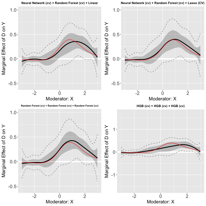

Application 1: Binary Treatment with Continuous Outcomes

In this section, we walk through an example application of DML estimator with binary treatment and continuous outcome. The data we are using is from Huddy, Mason, and Aarøe (2015), which explores the expressive model of partisanship, contrasting it with instrumental perspectives on political behavior. It argues that partisan identity, more than policy stances or ideological alignment, drives campaign involvement and emotional responses to political events. Key findings indicate that strongly identified partisans are more likely to engage in campaign activities and exhibit stronger emotional reactions—such as anger when threatened with electoral loss and positivity when victory seems likely—compared to those with weaker partisan identities.

The authors drew data from four studies conducted among populations that differ in their level of political activity: a highly engaged sample recruited from political blogs, and less politically engaged samples of students, New York (NY) State residents, and a national YouGov panel. The total number of respondents was 1,482. The variables of interest include

Outcome variable: level of anger (measured on a continuous scale from 0 to 1)
Treatment variable: the presence of an electoral loss threat (a binary yes/no variable)
Moderator Variable: strength of partisan identity (also measured on a continuous scale from 0 to 1)

Data overview

d <- app_hma2015
paged_table(head(d))

Y <- "totangry" 
D <- "threat" 
X <- "pidentity"
Z <- c("issuestr2", "pidstr2", "pidstr2_threat" ,"issuestr2_threat", "knowledge" , "educ" , "male" , "age10" )

Dlabel <- "Threat"
Xlabel <- "Partisan Identity"
Ylabel <- "Anger"
vartype <- "robust"
main <- "Huddy et al. (2015) \n APSR"
cl <- cuts <- cuts2 <- time <- NULL

Estimating marginal effects

out.dml.nn<-interflex(estimator='DML', data = d,
                      Y=Y,D=D,X=X, Z = Z, treat.type = "discrete",
                      model.y = 'nn', model.t = 'nn', 
                      Xlabel=Xlabel,Ylabel=Ylabel, Dlabel=Dlabel)
#> Baseline group not specified; choose treat = 0 as the baseline group.

lapply(out.dml.nn$est.dml, head, 20)
#> $`1`
#>             X           ME         sd lower CI(95%) upper CI(95%)
#> 1  0.08333334 -0.124049522 0.10847532  -0.336657241    0.08855820
#> 2  0.10204082 -0.094868947 0.09743050  -0.285829227    0.09609133
#> 3  0.12074830 -0.066957586 0.08707873  -0.237628756    0.10371359
#> 4  0.13945578 -0.040315438 0.07743184  -0.192079057    0.11144818
#> 5  0.15816327 -0.014942505 0.06850465  -0.149209153    0.11932414
#> 6  0.17687075  0.009161214 0.06031553  -0.109055061    0.12737749
#> 7  0.19557823  0.031995719 0.05288691  -0.071660719    0.13565216
#> 8  0.21428572  0.053561011 0.04624517  -0.037077860    0.14419988
#> 9  0.23299320  0.073857088 0.04041928  -0.005363246    0.15307742
#> 10 0.25170068  0.092883951 0.03543661   0.023429475    0.16233843
#> 11 0.27040817  0.110641600 0.03131422   0.049266857    0.17201634
#> 12 0.28911565  0.127130036 0.02804457   0.072163697    0.18209637
#> 13 0.30782313  0.142349257 0.02557814   0.092217016    0.19248150
#> 14 0.32653061  0.156299264 0.02381148   0.109629620    0.20296891
#> 15 0.34523810  0.168980058 0.02259085   0.124702808    0.21325731
#> 16 0.36394558  0.180391637 0.02173414   0.137793508    0.22298977
#> 17 0.38265306  0.190534002 0.02106076   0.149255662    0.23181234
#> 18 0.40136055  0.199407154 0.02041627   0.159391992    0.23942232
#> 19 0.42006803  0.207011091 0.01968617   0.168426908    0.24559527
#> 20 0.43877551  0.213345814 0.01880225   0.176494089    0.25019754
#>    lower uniform CI(95%) upper uniform CI(95%)
#> 1            -0.54487601             0.2967770
#> 2            -0.47284744             0.2831095
#> 3            -0.40477669             0.2708615
#> 4            -0.34070976             0.2600789
#> 5            -0.28070408             0.2508191
#> 6            -0.22483095             0.2431534
#> 7            -0.17317734             0.2371688
#> 8            -0.12584564             0.2329677
#> 9            -0.08294820             0.2306624
#> 10           -0.04459122             0.2303591
#> 11           -0.01084090             0.2321241
#> 12            0.01833205             0.2359280
#> 13            0.04311968             0.2415788
#> 14            0.06392340             0.2486751
#> 15            0.08133959             0.2566205
#> 16            0.09607475             0.2647085
#> 17            0.10882945             0.2722386
#> 18            0.12020288             0.2786114
#> 19            0.13063924             0.2833829
#> 20            0.14040311             0.2862885

Comparison of estimators


out.dml.nn<-interflex(estimator='DML', data = d,
                      model.y = 'nn', model.t = 'nn',
                      Y=Y,D=D,X=X, Z = Z, treat.type = "discrete",
                      Xlabel=Xlabel,
                      Ylabel=Ylabel, Dlabel=Dlabel,ylim=c(-0.4,1))
#> Baseline group not specified; choose treat = 0 as the baseline group.

out.dml.rf<-interflex(estimator='DML', data = d, 
                      model.y = 'rf', model.t = 'rf', 
                      Y=Y,D=D,X=X, Z = Z, treat.type = "discrete",
                      Xlabel=Xlabel,
                      Ylabel=Ylabel, Dlabel=Dlabel,ylim=c(-0.4,1))
#> Baseline group not specified; choose treat = 0 as the baseline group.

out.dml.hgb<-interflex(estimator='DML', data = d, 
                       model.y = 'hgb', model.t = 'hgb', 
                       Y=Y,D=D,X=X, Z = Z, treat.type = "discrete",
                       Xlabel=Xlabel,
                       Ylabel=Ylabel, Dlabel=Dlabel,ylim=c(-0.4,1))
#> Baseline group not specified; choose treat = 0 as the baseline group.

out.raw <- interflex(estimator = "raw", Y=Y,D=D,X=X,data=d, Xlabel=Xlabel,
                     Ylabel=Ylabel, Dlabel=Dlabel)
#> Baseline group not specified; choose treat = 0 as the baseline group.

out.est1<-interflex(estimator = "binning",Y=Y,D=D,X=X,Z=Z,data=d,
                    Xlabel=Xlabel, Ylabel=Ylabel, Dlabel=Dlabel,
                    nbins=3, cutoffs=cuts,  cl=cl, time=time,
                    pairwise=TRUE,  Xdistr = "histogram",ylim=c(-0.4,1))
#> Baseline group not specified; choose treat = 0 as the baseline group.

out.kernel<-interflex(estimator = "kernel", data=d, Y=Y,D=D,X=X,Z=Z,
                      cl=NULL, vartype = 'bootstrap', nboots = 2000, 
                      parallel = T, cores = 31,
                      Dlabel=Dlabel, Xlabel=Xlabel, Ylabel=Ylabel,
                      bw=0.917, Xdistr = "histogram", ylim=c(-0.4,1))
#> Baseline group not specified; choose treat = 0 as the baseline group. 
#> Number of evaluation points:50
#> Parallel computing with 20 cores...
#>

ggarrange(out.raw, out.est1$figure, out.kernel$figure,
          out.dml.nn$figure, out.dml.rf$figure, out.dml.hgb$figure, 
          common.legend = TRUE, legend = "none",
          labels = c("Raw", "Binning", "Kernel", 
                     "DML: nn","DML: rf", "DML: hgb"))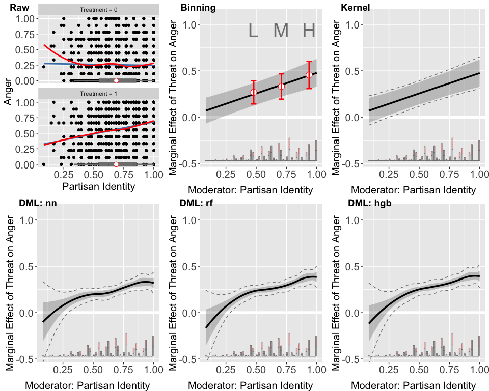

The lower left panel features a diagnostic scatterplot, illustrating that the relationship between anger and partisan identity is closely approximated by a linear fit in both treated and untreated groups, as indicated by the proximity of the linear and LOESS lines. This supports the assumption of a nearly linear interaction effect, with the impact of the threat on anger intensifying as partisan identity increases. Furthermore, the box plots demonstrate ample sufficient support for partisan identity ranging from approximately 0.3 to 1.

The three DML estimator plots consistently show that the marginal effect of the threat on anger escalates with increasing partisan identity across all machine learning methods employed. However, these DML estimators appear to overfit when partisan identity is below 0.25, a region with sparse data representation. The widen confidence intervals in areas where partisan identity is lower (e.g., below 0.25) further indicate uncertainty in the model’s estimations in these areas.

Application 2: Continuous Treatment with Continuous Outcomes

In this section, we demonstrate the application of the DML estimator, focusing on scenarios with continuous treatment and outcome variables. We refer to the study by Vernby (2013), which examines the impact of non-citizen suffrage on public policy in Swedish municipalities. Vernby’s analysis reveals that municipalities with a higher percentage of school-aged non-citizens would see a more significant increase in education spending following the enfranchisement of non-citizens.

In the example, the dataset consists of 183 cases. The key variables include:

Outcome Variable: Spending on education and social services.
Treatment Variable: Share of non-citizens in the municipal electorate.
Moderator Variable: Proportion of school-aged non-citizens.

Data overview

d <- app_vernby2013
paged_table(head(d))


Y <- "school_diff" 
D <- "noncitvotsh" 
X <- "noncit15" 
Z <- c("Taxbase2" ,  "Taxbase2_2" , "pop" , "pop_2" ,   "manu" , "manu_2")

Dlabel <- "Share NC"
Xlabel <- "Prop. School-Aged NC"
Ylabel <- "Δ Ed. Services"
vartype <- "robust"
name <- "vernby_2013a"
main <- "Vernby (2013) \n AJPS"
time <- cl <- cuts <- cuts2 <- NULL

Estimating marginal effects

out.dml.nn<-interflex(estimator='DML', data = d, 
          Y=Y,D=D,X=X, Z = Z, treat.type = "continuous",
          model.y = 'nn', model.t = 'nn',
          Xlabel=Xlabel,
          Ylabel=Ylabel, Dlabel=Dlabel)

lapply(out.dml.nn$est.dml, head, 20)
#> $`noncitvotsh=0.021 (50%)`
#>            X         ME        sd lower CI(95%) upper CI(95%)
#> 1  0.1180542 -3.1711311 3.0022757     -9.055483     2.7132211
#> 2  0.1232962 -3.2449677 1.9000995     -6.969094     0.4791589
#> 3  0.1285383 -3.2377741 0.9673659     -5.133776    -1.3417718
#> 4  0.1337804 -3.1495505 0.3947758     -3.923297    -2.3758041
#> 5  0.1390225 -2.9802969 0.7517866     -4.453772    -1.5068223
#> 6  0.1442645 -2.7300133 1.2598303     -5.199235    -0.2607913
#> 7  0.1495066 -2.3986996 1.6655044     -5.663028     0.8656292
#> 8  0.1547487 -1.9863558 1.9509458     -5.810139     1.8374276
#> 9  0.1599908 -1.4929820 2.1198001     -5.647714     2.6617497
#> 10 0.1652328 -0.9185782 2.1850034     -5.201106     3.3639497
#> 11 0.1704749 -0.2631443 2.1714550     -4.519118     3.9928292
#> 12 0.1757170  0.4733196 2.1241862     -3.690009     4.6366480
#> 13 0.1809591  1.2908135 2.1188424     -2.862041     5.4436683
#> 14 0.1862011  2.1893375 2.2583881     -2.237022     6.6156969
#> 15 0.1914432  3.1688916 2.6318205     -1.989382     8.3271649
#> 16 0.1966853  3.9957604 3.1156232     -2.110749    10.1022697
#> 17 0.2019273  3.8296881 3.0817340     -2.210400     9.8697758
#> 18 0.2071694  2.5952421 2.4472680     -2.201315     7.3917993
#> 19 0.2124115  0.2965205 1.5614830     -2.763930     3.3569709
#> 20 0.2176536 -1.5475746 1.6805451     -4.841382     1.7462333
#>    lower uniform CI(95%) upper uniform CI(95%)
#> 1             -14.407265             8.0650025
#> 2             -10.356164             3.8662286
#> 3              -6.858179             0.3826304
#> 4              -4.627015            -1.6720866
#> 5              -5.793887            -0.1667064
#> 6              -7.444977             1.9849506
#> 7              -8.631915             3.8345157
#> 8              -9.287846             5.3151346
#> 9              -9.426416             6.4404522
#> 10             -9.096038             7.2588820
#> 11             -8.389899             7.8636104
#> 12             -7.476530             8.4231690
#> 13             -6.639037             9.2206637
#> 14             -6.262768            10.6414430
#> 15             -6.680799            13.0185820
#> 16             -7.664581            15.6561016
#> 17             -7.703821            15.3631976
#> 18             -6.563754            11.7542380
#> 19             -5.547390             6.1404314
#> 20             -7.837080             4.7419309

Comparison of estimators


out.dml.nn<-interflex(estimator='DML', data = d, 
          Y=Y,D=D,X=X, Z = Z, treat.type = "continuous",
          model.y = 'nn', model.t = 'nn', 
          Xlabel=Xlabel, xlim = c(0.125,0.3),ylim = c(-25,75),
          Ylabel=Ylabel, Dlabel=Dlabel)

out.dml.rf<-interflex(estimator='DML', data = d, 
                       Y=Y,D=D,X=X, Z = Z, treat.type = "continuous",
                       model.y = 'rf', model.t = 'rf', 
                       Xlabel=Xlabel,xlim = c(0.125,0.3),ylim = c(-25,75),
                       Ylabel=Ylabel, Dlabel=Dlabel)

out.dml.hgb<-interflex(estimator='DML', data = d, 
                       Y=Y,D=D,X=X, Z = Z, treat.type = "continuous",
                       model.y = 'hgb', model.t = 'hgb', 
                       Xlabel=Xlabel,xlim = c(0.125,0.3),ylim = c(-25,75),
                       Ylabel=Ylabel, Dlabel=Dlabel)

out.raw <- interflex(estimator = "raw", Y=Y,D=D,X=X,data=d,Xlabel=Xlabel,
                     Ylabel=Ylabel, Dlabel=Dlabel, cutoffs=cuts,span=NULL)


out.est1<-interflex(estimator = "binning",Y=Y,D=D,X=X,Z=Z,data=d,
                    Xlabel=Xlabel, Ylabel=Ylabel, Dlabel=Dlabel,
                    cutoffs=cuts,  cl=cl, time=time,xlim = c(0.125,0.3),
                    pairwise=TRUE, Xdistr = "histogram")


out.kernel<-interflex(estimator = "kernel", data=d, Y=Y,D=D,X=X,Z=Z,
                      cl=cl,vartype = 'bootstrap', nboots = 2000, 
                      parallel = T, cores = 31,xlim = c(0.125,0.3),
                      Dlabel=Dlabel, Xlabel=Xlabel, Ylabel=Ylabel,
                      Xdistr = "histogram")
#> Cross-validating bandwidth ... 
#> Parallel computing with 20 cores...
#> Optimal bw=0.2569.
#> Number of evaluation points:50
#> Parallel computing with 20 cores...
#>

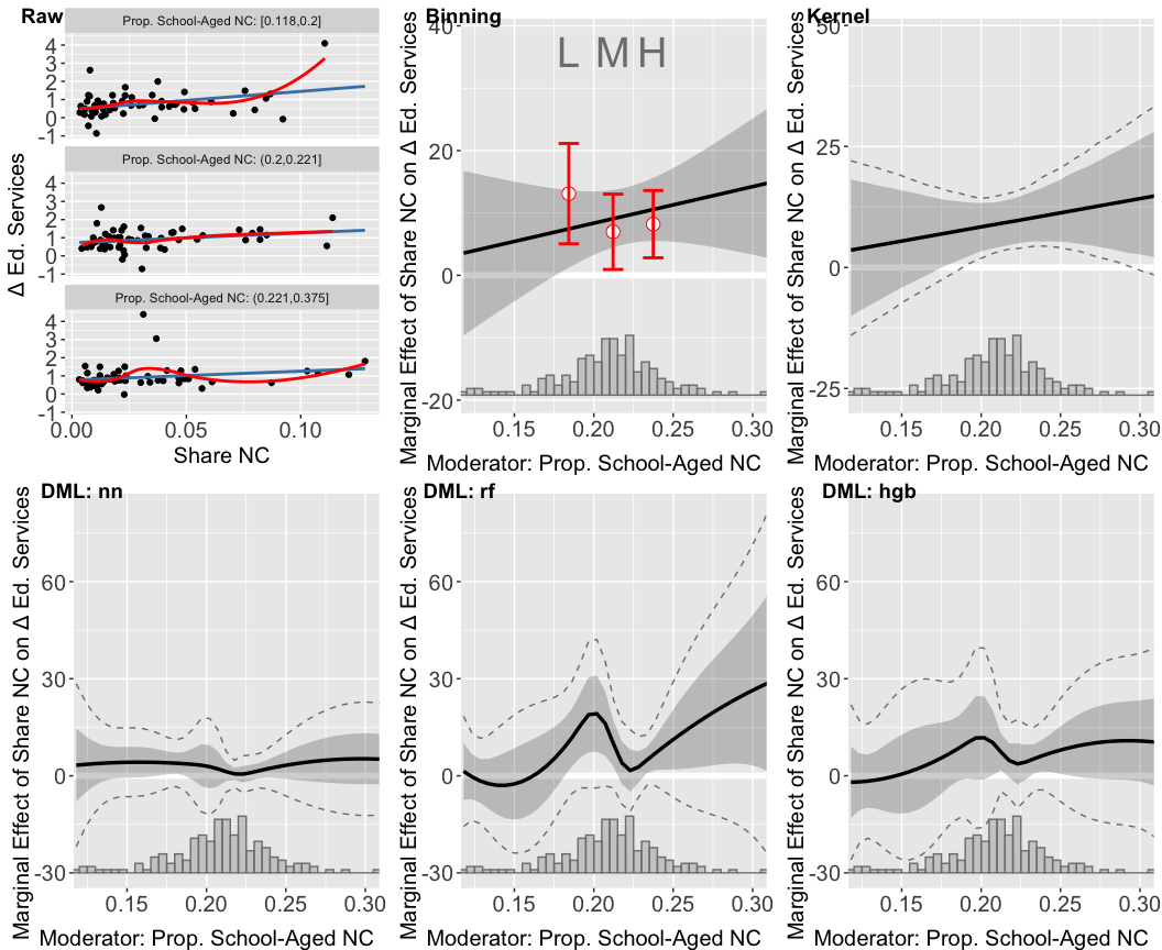
ggarrange(out.raw, 
          out.est1$figure, 
          out.kernel$figure,
          out.dml.nn$figure, 
          out.dml.rf$figure, out.dml.hgb$figure, 
          common.legend = TRUE, legend = "none",
          labels = c("Raw", "Binning", "Kernel", "DML: nn","DML: rf","DML: hgb"))

References

Bonvini, Matteo, Zhenghao Zeng, Miaoqing Yu, Edward H Kennedy, and Luke Keele. 2023. “Flexibly Estimating and Interpreting Heterogeneous Treatment Effects of Laparoscopic Surgery for Cholecystitis Patients.” arXiv Preprint arXiv:2311.04359.

Chernozhukov, Victor, Denis Chetverikov, Mert Demirer, Esther Duflo, Christian Hansen, Whitney Newey, and James Robins. 2018. “Double/Debiased Machine Learning for Treatment and Structural Parameters.” Oxford University Press Oxford, UK.

Huddy, Leonie, Lilliana Mason, and Lene Aarøe. 2015. “Expressive Partisanship: Campaign Involvement, Political Emotion, and Partisan Identity.” American Political Science Review 109 (1): 1–17.

Rubin, Donald B. 1974. “Estimating Causal Effects of Treatments in Randomized and Nonrandomized Studies.” Journal of Educational Psychology 66 (5): 688.

Semenova, Vira, and Victor Chernozhukov. 2021. “Debiased Machine Learning of Conditional Average Treatment Effects and Other Causal Functions.” The Econometrics Journal 24 (2): 264–89.

Vernby, Kåre. 2013. “Inclusion and Public Policy: Evidence from Sweden’s Introduction of Noncitizen Suffrage.” American Journal of Political Science 57 (1): 15–29.