Interflex with Discrete Outcomes
discrete.RmdLoad the package as well as the simulated toy datasets for this tutorial. s1-s5 are for the tutorial for interflex with continuous outcomes. The response variable Y in s6-s9 are all binary(0/1), and the link function is logit.
library(interflex)
data(interflex)
ls()
#>  [1] "app_hma2015"    "app_vernby2013" "s1"             "s2"
#>  [5] "s3"             "s4"             "s5"             "s6"
#>  [9] "s7"             "s8"             "s9"
s6 is a case of a dichotomous treatment indicator with the DGP , where D is binary too.
s7 is a case of a continuous treatment indicator with the same DGP as s6 except that D is continuous;
s8 is a case of a dichotomous treatment indicator with nonlinear “linear predictor”:
s9 is a case of a discrete treatment indicator in which for the group 0, , for the group 1 , and for the group 2, .
set.seed(110)
n <- 2000
x <- runif(n,min=-3, max = 3)
d1 <- sample(x = c(0,1),size = n,replace = T)
d2 <- runif(min = 0,max = 1,n = n)
d3 <- sample(x = c(0,1,2),size = n,replace = T)
Z1 <- runif(min = 0,max = 1,n = n)
Z2 <- rnorm(n,3,1)

## s6
link1 <- -1+d1+x+d1*x
prob1 <- exp(link1)/(1+exp(link1))
rand.u <- runif(min = 0,max = 1,n = n)
y1 <- as.numeric(rand.u<prob1)
s6 <- cbind.data.frame(X=x,D=d1,Z1=Z1,Z2=Z2,Y=y1)

## s7
link2 <- -1+d2+x+d2*x
prob2 <- exp(link2)/(1+exp(link2))
rand.u <- runif(min = 0,max = 1,n = n)
y2 <- as.numeric(rand.u<prob2)
s7 <- cbind.data.frame(X=x,D=d2,Z1=Z1,Z2=Z2,Y=y2)

## s8
link3 <- -1+d1+x+d1*x-d1*x*x
prob3 <- exp(link3)/(1+exp(link3))
rand.u <- runif(min = 0,max = 1,n = n)
y3 <- as.numeric(rand.u<prob3)
s8 <- cbind.data.frame(X=x,D=d1,Z1=Z1,Z2=Z2,Y=y3)

## s9
link4 <- rep(NA,n)
link4[which(d3==0)] <- -x[which(d3==0)]
link4[which(d3==1)] <- (1+x)[which(d3==1)]
link4[which(d3==2)] <- (4-x*x-x)[which(d3==2)]

prob4 <- exp(link4)/(1+exp(link4))
rand.u <- runif(min = 0,max = 1,n = n)
y4 <- as.numeric(rand.u<prob4)
s9 <- cbind.data.frame(X=x,D=d3,Z1=Z1,Z2=Z2,Y=y4)
Linear linear predictors
When setting the option estimator to “linear”, the
program will conduct the classic glm regression and estimate the CME
using the coefficients from the regression. In the following command,
the outcome variable is “Y”, the moderator is “X”, the covariates are
“Z1” and “Z2”, and here it uses logit link function.
s6.linear <- interflex(estimator='linear', method='logit', data = s6,
                       Y = "Y", D = "D", X = "X",Z = c("Z1", "Z2"))
Marginal/treatment effects
The estimated CME of D on Y across the
support of X are saved in
s6.linear$est.lin
#> $`1`
#>                 X           ME          sd lower CI(95%) upper CI(95%)
#>  [1,] -2.99866836 -0.019251870 0.005003764   -0.02906502 -0.0094387158
#>  [2,] -2.87637418 -0.021317834 0.005449665   -0.03200547 -0.0106301994
#>  [3,] -2.75408000 -0.023544378 0.005931826   -0.03517760 -0.0119111516
#>  [4,] -2.63178582 -0.025923811 0.006453763   -0.03858064 -0.0132669844
#>  [5,] -2.50949164 -0.028439744 0.007019848   -0.04220675 -0.0146727390
#>  [6,] -2.38719747 -0.031063958 0.007635613   -0.04603857 -0.0160893418
#>  [7,] -2.26490329 -0.033752401 0.008308139   -0.05004594 -0.0174588567
#>  [8,] -2.14260911 -0.036440155 0.009046485   -0.05418171 -0.0186986021
#>  [9,] -2.02031493 -0.039035211 0.009862119   -0.05837635 -0.0196940734
#> [10,] -1.89802075 -0.041410927 0.010769254   -0.06253110 -0.0202907565
#> [11,] -1.77572658 -0.043397172 0.011784900   -0.06650918 -0.0202851641
#> [12,] -1.65343240 -0.044770349 0.012928383   -0.07012490 -0.0194157938
#> [13,] -1.53113822 -0.045242878 0.014220025   -0.07313054 -0.0173552141
#> [14,] -1.40884404 -0.044453331 0.015678635   -0.07520156 -0.0137051061
#> [15,] -1.28654986 -0.041959296 0.017317600   -0.07592178 -0.0079968083
#> [16,] -1.16425569 -0.037236352 0.019139603   -0.07477207  0.0002993653
#> [17,] -1.04196151 -0.029687959 0.021130481   -0.07112809  0.0117521765
#> [18,] -0.91966733 -0.018672518 0.023253355   -0.06427594  0.0269309016
#> [19,] -0.79737315 -0.003554373 0.025444930   -0.05345581  0.0463470624
#> [20,] -0.67507897  0.016216108 0.027616301   -0.03794372  0.0703759387
#> [21,] -0.55278480  0.040993593 0.029660368   -0.01717497  0.0991621536
#> [22,] -0.43049062  0.070810436 0.031466139    0.00910048  0.1325203922
#> [23,] -0.30819644  0.105255369 0.032936905    0.04066101  0.1698497246
#> [24,] -0.18590226  0.143395507 0.034005693    0.07670509  0.2100859215
#> [25,] -0.06360808  0.183781862 0.034640990    0.11584553  0.2517181913
#> [26,]  0.05868609  0.224563486 0.034840902    0.15623510  0.2928918742
#> [27,]  0.18098027  0.263702051 0.034622433    0.19580211  0.3316019877
#> [28,]  0.30327445  0.299240241 0.034016324    0.23252898  0.3659515048
#> [29,]  0.42556863  0.329554334 0.033071755    0.26469552  0.3944131526
#> [30,]  0.54786281  0.353527826 0.031864584    0.29103646  0.4160191961
#> [31,]  0.67015698  0.370614879 0.030498613    0.31080239  0.4304273685
#> [32,]  0.79245116  0.380801084 0.029094651    0.32374198  0.4378601862
#> [33,]  0.91474534  0.384495639 0.027770455    0.33003349  0.4389577883
#> [34,]  1.03703952  0.382396089 0.026619316    0.33019150  0.4346006774
#> [35,]  1.15933370  0.375358554 0.025694929    0.32496683  0.4257502769
#> [36,]  1.28162787  0.364292254 0.025007011    0.31524964  0.4133348643
#> [37,]  1.40392205  0.350084305 0.024527753    0.30198159  0.3981870148
#> [38,]  1.52621623  0.333552576 0.024205192    0.28608246  0.3810226944
#> [39,]  1.64851041  0.315420701 0.023977962    0.26839621  0.3624451871
#> [40,]  1.77080459  0.296308711 0.023787071    0.24965859  0.3429588292
#> [41,]  1.89309876  0.276733695 0.023583020    0.23048375  0.3229836381
#> [42,]  2.01539294  0.257116296 0.023328736    0.21136504  0.3028675499
#> [43,]  2.13768712  0.237790180 0.022999661    0.19268429  0.2828960663
#> [44,]  2.25998130  0.219012671 0.022582311    0.17472527  0.2633000700
#> [45,]  2.38227548  0.200975468 0.022072233    0.15768841  0.2442625245
#> [46,]  2.50456965  0.183814835 0.021471872    0.14170518  0.2259244904
#> [47,]  2.62686383  0.167620965 0.020788618    0.12685127  0.2083906543
#> [48,]  2.74915801  0.152446375 0.020033131    0.11315831  0.1917344381
#> [49,]  2.87145219  0.138313304 0.019217967    0.10062390  0.1760027040
#> [50,]  2.99374637  0.125220123 0.018356499    0.08922019  0.1612200505
#>       lower uniform CI(95%) upper uniform CI(95%)
#>  [1,]           -0.03228029          -0.006223452
#>  [2,]           -0.03550725          -0.007128414
#>  [3,]           -0.03898921          -0.008099545
#>  [4,]           -0.04272763          -0.009119996
#>  [5,]           -0.04671749          -0.010162003
#>  [6,]           -0.05094498          -0.011182934
#>  [7,]           -0.05538450          -0.012120304
#>  [8,]           -0.05999470          -0.012885612
#>  [9,]           -0.06471344          -0.013356982
#> [10,]           -0.06945109          -0.013370768
#> [11,]           -0.07408179          -0.012712554
#> [12,]           -0.07843228          -0.011108417
#> [13,]           -0.08226789          -0.008217868
#> [14,]           -0.08527616          -0.003630502
#> [15,]           -0.08704954           0.003130944
#> [16,]           -0.08707058           0.012597880
#> [17,]           -0.08470588           0.025329967
#> [18,]           -0.07921782           0.041872785
#> [19,]           -0.06980593           0.062697184
#> [20,]           -0.05568910           0.088121316
#> [21,]           -0.03623380           0.118220985
#> [22,]           -0.01111868           0.152739556
#> [23,]            0.01949678           0.191013957
#> [24,]            0.05485409           0.231936924
#> [25,]            0.09358631           0.273977416
#> [26,]            0.13384742           0.315279556
#> [27,]            0.17355481           0.353849288
#> [28,]            0.21067114           0.387809338
#> [29,]            0.24344463           0.415664036
#> [30,]            0.27056126           0.436494389
#> [31,]            0.29120493           0.450024830
#> [32,]            0.30504666           0.456555505
#> [33,]            0.31218906           0.456802220
#> [34,]            0.31308675           0.451705423
#> [35,]            0.30845607           0.442261040
#> [36,]            0.29918091           0.429403593
#> [37,]            0.28622082           0.413947787
#> [38,]            0.27052895           0.396576199
#> [39,]            0.25298872           0.377852681
#> [40,]            0.23437376           0.358243662
#> [41,]            0.21533004           0.338137354
#> [42,]            0.19637472           0.317857871
#> [43,]            0.17790543           0.297674934
#> [44,]            0.16021458           0.277810762
#> [45,]            0.14350548           0.258445456
#> [46,]            0.12790802           0.239721648
#> [47,]            0.11349315           0.221748775
#> [48,]            0.10028565           0.204607106
#> [49,]            0.08827504           0.188351573
#> [50,]            0.07742488           0.173015366
Users can then use the command plot to visualize the treatment effects and their point-wise confidence interval. We also report the uniform/simultaneous confidence interval, as depicted by the dashed lines.
s6.plot <- plot(s6.linear)
s6.plot
When setting the option show.all to
TRUE in the command plot, the program
will return a list in which every element is the plot of one treated
group. As all of them are ggplot2 objects, users can then edit those
graphs in their ways. For example, we can add the “true” treatment
effects to the plot as a comparison.
library(ggplot2)
s6.linear.plot <- plot.interflex(s6.linear,show.all = TRUE, Xdistr = 'none')$`1`
TE <- exp(-1+1+x+1*x)/(1+exp(-1+1+x+1*x))-exp(-1+0+x+0*x)/(1+exp(-1+0+x+0*x))
s6.linear.plot + geom_line(aes(x=x,y=TE),color='red')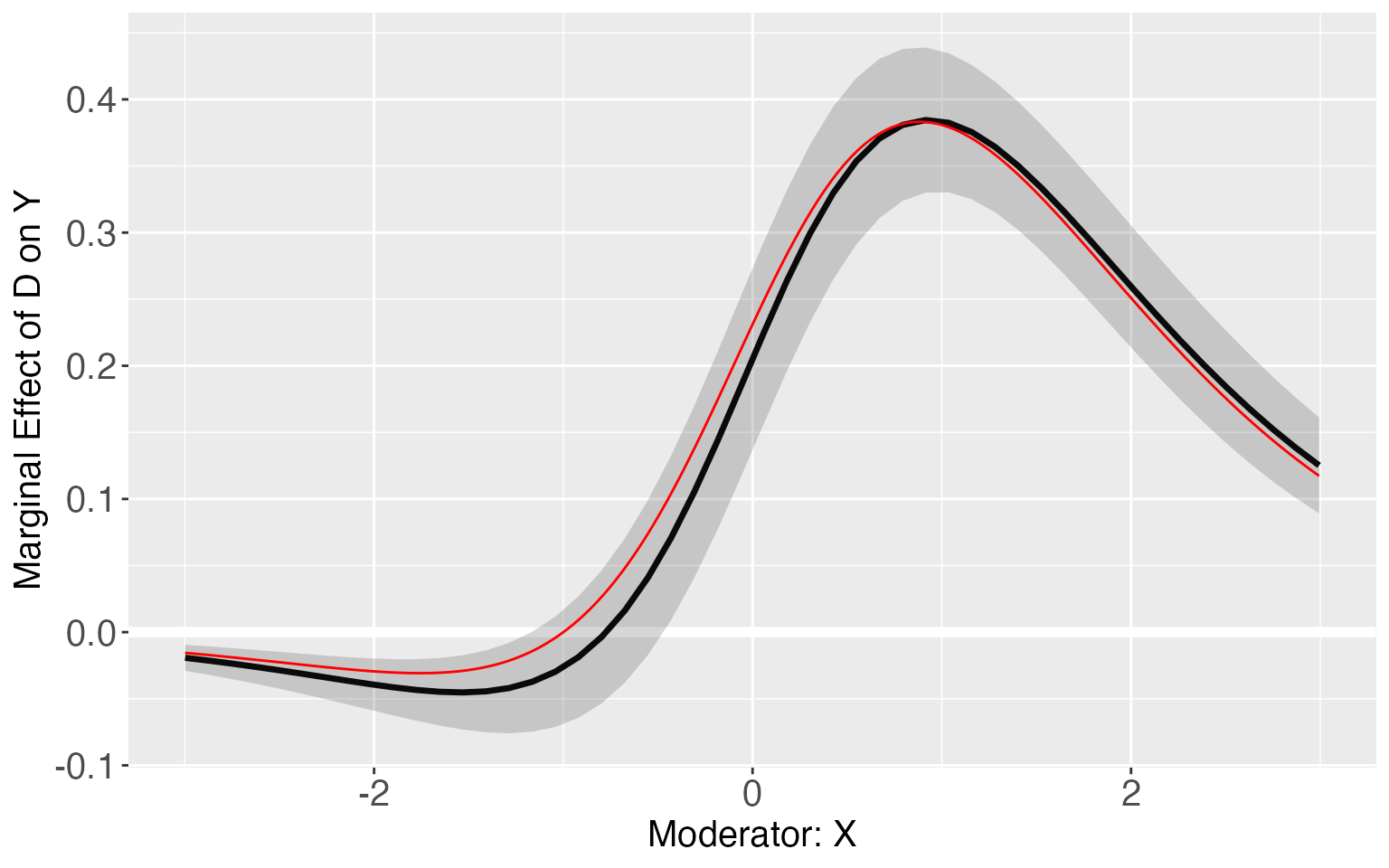
E(Y|X,Z,D)
The estimated are saved in
s6.linear$pred.lin
#> $`1`
#> X E(Y) sd lower CI(95%) upper CI(95%)
#> [1,] -2.99866836 0.001656739 0.0006647875 0.0003529877 0.002960490
#> [2,] -2.87637418 0.002143747 0.0008283440 0.0005192363 0.003768257
#> [3,] -2.75408000 0.002773516 0.0010305164 0.0007525143 0.004794518
#> [4,] -2.63178582 0.003587628 0.0012798092 0.0010777245 0.006097532
#> [5,] -2.50949164 0.004639595 0.0015863495 0.0015285183 0.007750671
#> [6,] -2.38719747 0.005998163 0.0019620835 0.0021502143 0.009846112
#> [7,] -2.26490329 0.007751450 0.0024209368 0.0030036189 0.012499281
#> [8,] -2.14260911 0.010012067 0.0029788982 0.0041699877 0.015854146
#> [9,] -2.02031493 0.012923380 0.0036539626 0.0057573950 0.020089364
#> [10,] -1.89802075 0.016666993 0.0044658428 0.0079087855 0.025425200
#> [11,] -1.77572658 0.021471457 0.0054353268 0.0108119419 0.032130972
#> [12,] -1.65343240 0.027621964 0.0065831182 0.0147114524 0.040532475
#> [13,] -1.53113822 0.035470421 0.0079279712 0.0199224458 0.051018397
#> [14,] -1.40884404 0.045444704 0.0094839317 0.0268452495 0.064044158
#> [15,] -1.28654986 0.058054936 0.0112565582 0.0359790872 0.080130785
#> [16,] -1.16425569 0.073893446 0.0132381803 0.0479313307 0.099855562
#> [17,] -1.04196151 0.093623523 0.0154026125 0.0634166218 0.123830424
#> [18,] -0.91966733 0.117950719 0.0177003132 0.0832376722 0.152663766
#> [19,] -0.79737315 0.147569937 0.0200556848 0.1082376421 0.186902231
#> [20,] -0.67507897 0.183083150 0.0223687468 0.1392145839 0.226951716
#> [21,] -0.55278480 0.224888036 0.0245231771 0.1767942995 0.272981773
#> [22,] -0.43049062 0.273048017 0.0264009744 0.2212716298 0.324824404
#> [23,] -0.30819644 0.327168258 0.0279005805 0.2724509122 0.381885604
#> [24,] -0.18590226 0.386315009 0.0289516784 0.3295362975 0.443093720
#> [25,] -0.06360808 0.449018643 0.0295194291 0.3911264849 0.506910802
#> [26,] 0.05868609 0.513385676 0.0295964275 0.4553425119 0.571428840
#> [27,] 0.18098027 0.577311765 0.0291897202 0.5200662167 0.634557313
#> [28,] 0.30327445 0.638749245 0.0283143973 0.5832203406 0.694278150
#> [29,] 0.42556863 0.695959742 0.0269987629 0.6430109996 0.748908485
#> [30,] 0.54786281 0.747688830 0.0252947555 0.6980819093 0.797295751
#> [31,] 0.67015698 0.793231587 0.0232827714 0.7475704773 0.838892697
#> [32,] 0.79245116 0.832396511 0.0210655245 0.7910837644 0.873709257
#> [33,] 0.91474534 0.865401811 0.0187538612 0.8286225938 0.902181029
#> [34,] 1.03703952 0.892745021 0.0164513135 0.8604814549 0.925008587
#> [35,] 1.15933370 0.915078619 0.0142427979 0.8871462938 0.943010945
#> [36,] 1.28162787 0.933110159 0.0121894060 0.9092048515 0.957015466
#> [37,] 1.40392205 0.947532546 0.0103284802 0.9272768011 0.967788290
#> [38,] 1.52621623 0.958981960 0.0086770061 0.9419650111 0.975998908
#> [39,] 1.64851041 0.968017223 0.0072363999 0.9538255260 0.982208921
#> [40,] 1.77080459 0.975113889 0.0059973414 0.9633521766 0.986875601
#> [41,] 1.89309876 0.980667323 0.0049439269 0.9709715185 0.990363127
#> [42,] 2.01539294 0.985000548 0.0040568821 0.9770443760 0.992956721
#> [43,] 2.13768712 0.988374039 0.0033158494 0.9818711467 0.994876932
#> [44,] 2.25998130 0.990995742 0.0027008945 0.9856988711 0.996292613
#> [45,] 2.38227548 0.993030409 0.0021934126 0.9887287883 0.997332030
#> [46,] 2.50456965 0.994607810 0.0017766026 0.9911236176 0.998092002
#> [47,] 2.62686383 0.995829702 0.0014356499 0.9930141714 0.998645234
#> [48,] 2.74915801 0.996775607 0.0011577229 0.9945051337 0.999046080
#> [49,] 2.87145219 0.997507499 0.0009318597 0.9956799781 0.999335020
#> [50,] 2.99374637 0.998073583 0.0007487971 0.9966050761 0.999542089
#>
#> $`0`
#> X E(Y) sd lower CI(95%) upper CI(95%)
#> [1,] -2.99866836 0.02090861 0.004959854 0.01118157 0.03063565
#> [2,] -2.87637418 0.02346158 0.005386879 0.01289708 0.03402608
#> [3,] -2.75408000 0.02631789 0.005842264 0.01486031 0.03777548
#> [4,] -2.63178582 0.02951144 0.006326348 0.01710449 0.04191838
#> [5,] -2.50949164 0.03307934 0.006839136 0.01966674 0.04649194
#> [6,] -2.38719747 0.03706212 0.007380228 0.02258835 0.05153589
#> [7,] -2.26490329 0.04150385 0.007948743 0.02591514 0.05709256
#> [8,] -2.14260911 0.04645222 0.008543234 0.02969762 0.06320682
#> [9,] -2.02031493 0.05195859 0.009161613 0.03399125 0.06992593
#> [10,] -1.89802075 0.05807792 0.009801071 0.03885651 0.07729933
#> [11,] -1.77572658 0.06486863 0.010458010 0.04435886 0.08537840
#> [12,] -1.65343240 0.07239231 0.011127991 0.05056860 0.09421602
#> [13,] -1.53113822 0.08071330 0.011805716 0.05756047 0.10386613
#> [14,] -1.40884404 0.08989803 0.012485037 0.06541295 0.11438312
#> [15,] -1.28654986 0.10001423 0.013159026 0.07420735 0.12582111
#> [16,] -1.16425569 0.11112980 0.013820112 0.08402642 0.13823317
#> [17,] -1.04196151 0.12331148 0.014460298 0.09495261 0.15167036
#> [18,] -0.91966733 0.13662324 0.015071478 0.10706574 0.16618073
#> [19,] -0.79737315 0.15112431 0.015645862 0.12044036 0.18180826
#> [20,] -0.67507897 0.16686704 0.016176511 0.13514241 0.19859168
#> [21,] -0.55278480 0.18389444 0.016657969 0.15122559 0.21656329
#> [22,] -0.43049062 0.20223758 0.017086964 0.16872741 0.23574776
#> [23,] -0.30819644 0.22191289 0.017463118 0.18766502 0.25616076
#> [24,] -0.18590226 0.24291950 0.017789579 0.20803139 0.27780761
#> [25,] -0.06360808 0.26523678 0.018073435 0.22979199 0.30068158
#> [26,] 0.05868609 0.28882219 0.018325761 0.25288254 0.32476184
#> [27,] 0.18098027 0.31360971 0.018561126 0.27720848 0.35001095
#> [28,] 0.30327445 0.33950900 0.018796424 0.30264631 0.37637169
#> [29,] 0.42556863 0.36640541 0.019049014 0.32904735 0.40376347
#> [30,] 0.54786281 0.39416100 0.019334305 0.35624345 0.43207856
#> [31,] 0.67015698 0.42261671 0.019663179 0.38405418 0.46117924
#> [32,] 0.79245116 0.45159543 0.020039752 0.41229438 0.49089647
#> [33,] 0.91474534 0.48090617 0.020460049 0.44078086 0.52103149
#> [34,] 1.03703952 0.51034893 0.020911912 0.46933744 0.55136042
#> [35,] 1.15933370 0.53972007 0.021376186 0.49779806 0.58164207
#> [36,] 1.28162787 0.56881790 0.021828873 0.52600812 0.61162769
#> [37,] 1.40392205 0.59744824 0.022243775 0.55382476 0.64107172
#> [38,] 1.52621623 0.62542938 0.022595139 0.58111683 0.66974194
#> [39,] 1.64851041 0.65259652 0.022859906 0.60776472 0.69742833
#> [40,] 1.77080459 0.67880518 0.023019369 0.63366064 0.72394971
#> [41,] 1.89309876 0.70393363 0.023060169 0.65870908 0.74915818
#> [42,] 2.01539294 0.72788425 0.022974669 0.68282738 0.77294113
#> [43,] 2.13768712 0.75058386 0.022760811 0.70594639 0.79522132
#> [44,] 2.25998130 0.77198307 0.022421584 0.72801088 0.81595526
#> [45,] 2.38227548 0.79205494 0.021964239 0.74897968 0.83513021
#> [46,] 2.50456965 0.81079297 0.021399373 0.76882550 0.85276045
#> [47,] 2.62686383 0.82820874 0.020739971 0.78753445 0.86888302
#> [48,] 2.74915801 0.84432923 0.020000497 0.80510517 0.88355329
#> [49,] 2.87145219 0.85919419 0.019196080 0.82154772 0.89684067
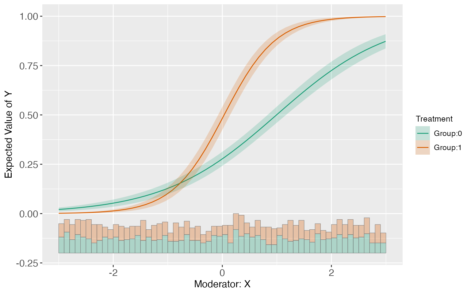
#> [50,] 2.99374637 0.87285346 0.018341824 0.83688231 0.90882461Users can then use the command predict to visualize
E(Y|X,Z,D). The option pool can help users draw E(Y|X,Z,D)
for different D in one plot.
Differences in effects
The difference of margnal effects/treatment effects at different
values of the moderator(by default are the 25%, 50%, 75% quantiles of
the moderator) are saved in “diff.estimate”. Users can also pass two or
three values(should be in the support of “X”) into
diff.values when applying linear estimator.
s6.linear.a <- interflex(estimator = 'linear', method='logit', data = s6,
                         Y = 'Y', D = 'D', diff.values = c(-2,0,2),
                         X = 'X', Z = c('Z1','Z2'))
plot.interflex(s6.linear.a,diff.values = c(-2,0,2))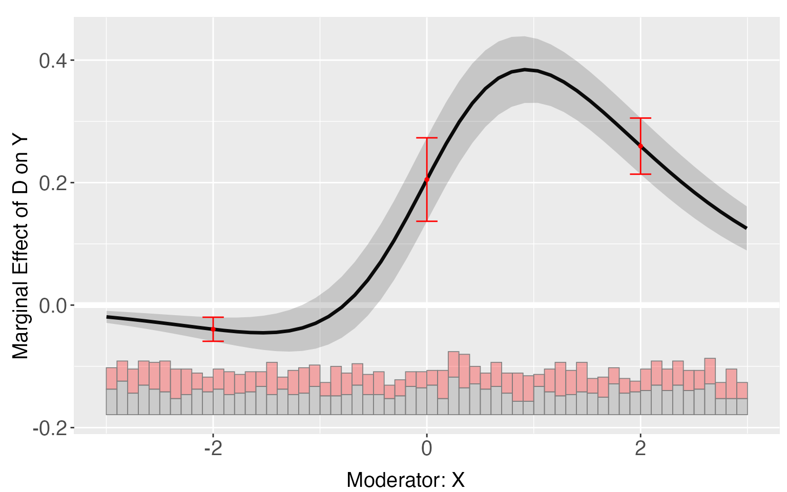
s6.linear.a$diff.estimate
#> $`1`
#>         diff.estimate    sd z-value p-value lower CI(95%) upper CI(95%)
#> 0 vs -2         0.245 0.031   7.994   0.000         0.185         0.305
#> 2 vs 0          0.055 0.038   1.447   0.148        -0.019         0.128
#> 2 vs -2         0.299 0.028  10.505   0.000         0.243         0.355
Average CME
The estimated average treatment effect (ATE) is saved in “Avg.estimate”. Here the program uses the coefficients from the regression and the input data to calculate the ATE/AME.
s6.linear$Avg.estimate
#> $`1`
#>                            ATE    sd z-value p-value lower CI(95%)
#> Average Treatment Effect 0.141 0.015   9.374   0.000         0.111
#>                          upper CI(95%)
#> Average Treatment Effect         0.170
Uncertainty estimates
In the default setting, confidence intervals of treatment effects, E(Y|D,X,Z), difference of treatment effects and ATE are all estimated using the delta method. The program also supports the bootstrap method and the simulation methods proposed by King(2000). For the sample dataset, the differences between these three methods are ignorable.
library(patchwork)
s6.linear.b <- interflex(estimator='linear', method='logit',
                         Y = "Y", D = "D", X = "X",Z = c("Z1", "Z2"),
                         data = s6, vartype='bootstrap')
s6.linear.c <- interflex(estimator='linear', method='logit',
                         Y = "Y", D = "D", X = "X",Z = c("Z1", "Z2"),
                         data = s6, vartype='simu')
s6.p1 <- plot(s6.linear,ylim=c(-0.3,0.6),main = 'delta')
s6.p2 <- plot(s6.linear.b,ylim=c(-0.3,0.6),main = 'bootstrap')
s6.p3 <- plot(s6.linear.c,ylim=c(-0.3,0.6),main = 'simu')
s6.p1+s6.p2+s6.p3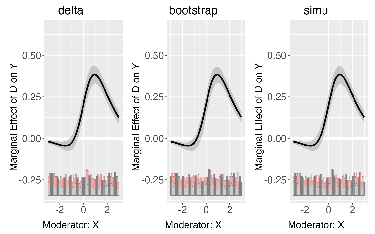
Note that the variance-covariance matrix of coefficients used by the
delta method or the simulation method by default is the robust standard
error matrix esimated from the regression. Users can also choose
“homoscedastic” or “cluster” standard error by specifying the option
vcov.type.
Set covariate values
Different from the linear case, the treatment effects in glm models
rely on the choice of values of all covariates. By default, all
covariates are set to their means when estimating TE, E(Y|X,D,Z) and
difference of TE. Users can also pass their preferred values of
covariates into the option Z.ref, which must have the same
length as Z.
s6.linear.d <- interflex(estimator='linear', method='logit',
                         Y = "Y", D = "D", X = "X",Z = c("Z1", "Z2"),
                         data = s6, Z.ref=c(1,1))
plot(s6.linear.d)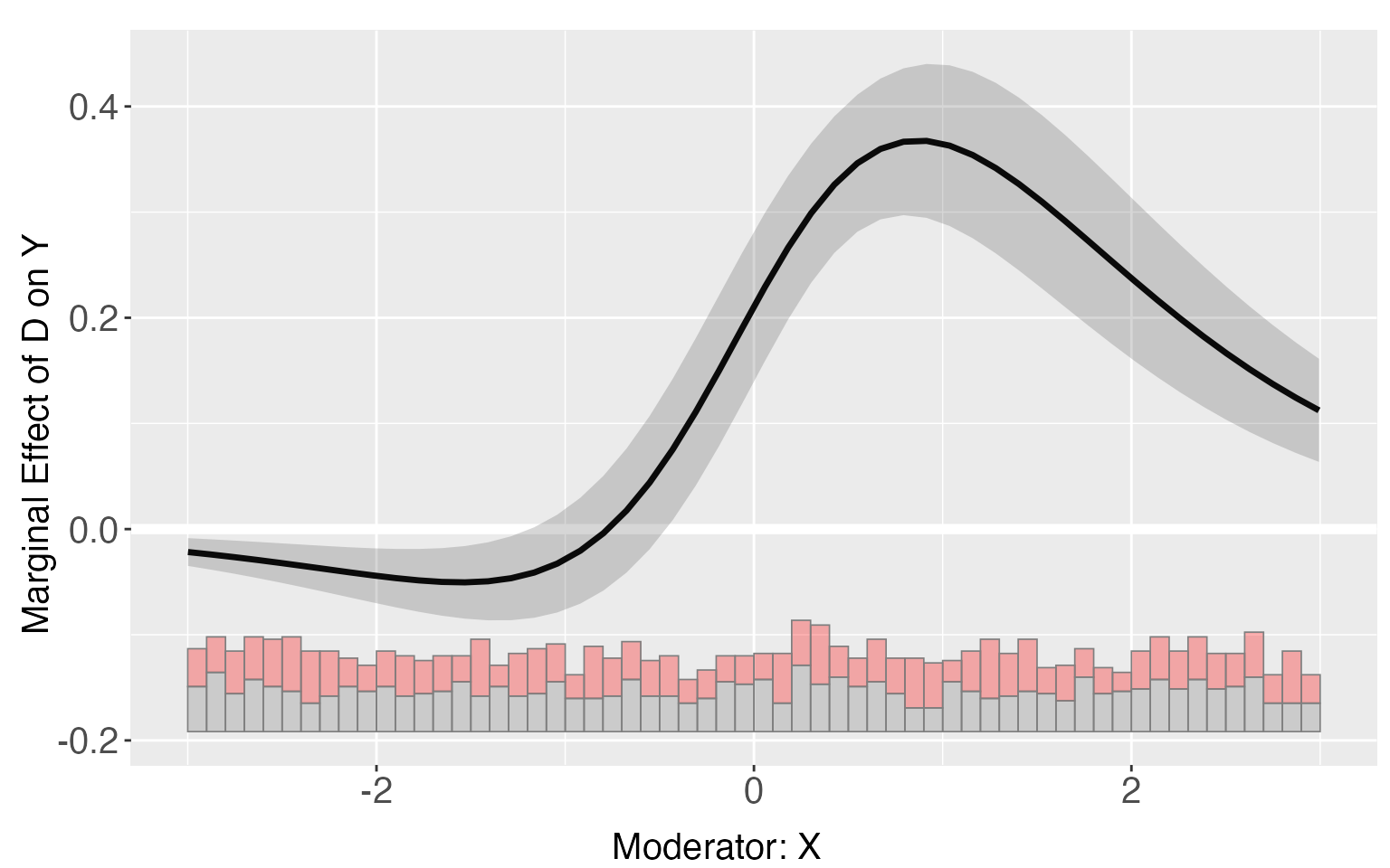
Fully moderated model
For the linear estimator, when the option full.moderate
is set to TRUE, interaction terms between the moderatoe
“X” and each covariate will enter the model, which is the case in
Blackwell and Olson (2020). This extension in some cases can reduce the
bias of the original model.
s6.linear.f <- interflex(estimator='linear', method='logit',
                         Y = "Y", D = "D", X = "X",Z = c("Z1", "Z2"),
                         data = s6, full.moderate=TRUE)
plot(s6.linear.f)
Continuous treatments
When the treatment variable D is continuous, the package
will choose the mean of D as the “reference value” when
estimating the CME,
and difference of CME.
s7.linear <- interflex(estimator = 'linear', method = 'logit', data = s7,
                       Y = 'Y', D = 'D',X = 'X',Z = c('Z1','Z2'))
plot(s7.linear)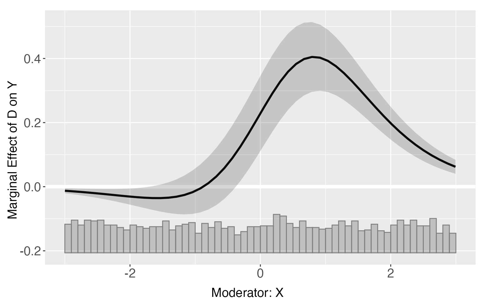
As the CME in glm models also depends on the value of D, users can
pass their preferred values of D into the option D.ref. For
example, we can set D to three values: 0.25, 0.5 and
0.75.
s7.linear.a <- interflex(estimator = 'linear', method='logit', data = s7,
                         Y = 'Y', D = 'D', X = 'X', Z = c('Z1','Z2'),
                         D.ref = c(0.25,0.5,0.75))
plot(s7.linear.a)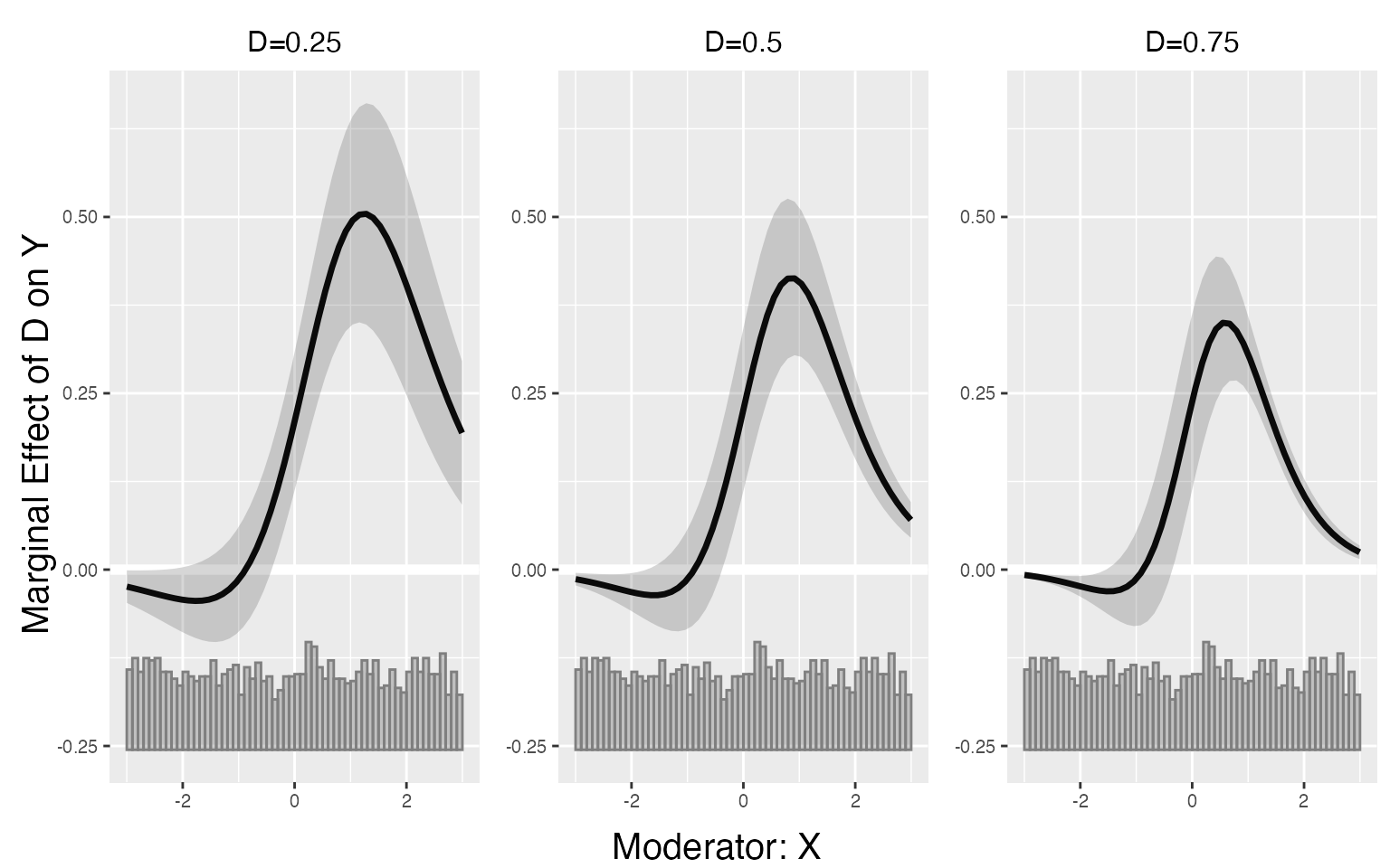
Predicted values and difference of CME are also grouped by D.ref.
predict(s7.linear.a)
s7.linear.a$diff.estimate
#> $`D=0.25`
#>            diff.estimate    sd z-value p-value lower CI(95%) upper CI(95%)
#> 50% vs 25%         0.264 0.037   7.056   0.000         0.191         0.337
#> 75% vs 50%         0.274 0.070   3.922   0.000         0.137         0.411
#> 75% vs 25%         0.538 0.092   5.826   0.000         0.357         0.719
#>
#> $`D=0.5`
#>            diff.estimate    sd z-value p-value lower CI(95%) upper CI(95%)
#> 50% vs 25%         0.275 0.047   5.840   0.000         0.182         0.367
#> 75% vs 50%         0.099 0.053   1.853   0.064        -0.006         0.203
#> 75% vs 25%         0.373 0.051   7.389   0.000         0.274         0.472
#>
#> $`D=0.75`
#>            diff.estimate    sd z-value p-value lower CI(95%) upper CI(95%)
#> 50% vs 25%         0.280 0.054   5.189   0.000         0.174         0.386
#> 75% vs 50%        -0.043 0.061  -0.708   0.479        -0.164         0.077
#> 75% vs 25%         0.236 0.023  10.070   0.000         0.190         0.282
The ATE is saved in “Avg.estimate”, which doesn’t rely on the choice of “D.ref”.
s7.linear.a$Avg.estimate
#>                           AME    sd z-value p-value lower CI(95%) upper CI(95%)
#> Average Marginal Effect 0.148 0.026   5.630   0.000         0.097         0.200
Users can also draw a Generalized Additive Model (GAM) plot, the usage is the same as the linear estimator.
s7.gam <- interflex(estimator='gam', method='logit', data=s7,
                    Y = 'Y', D = 'D', X = 'X', Z = c('Z1','Z2'),
                    CI=FALSE)
Limitations of the linear linear-predictor
When the “linear predictor” (the term in the bracket of ) actually doesn’t take a linear form, such as in s8, the simple linear estimator may suffer from severe bias.
s8.linear <- interflex(estimator='linear',data=s8,Y='Y',D='D', X='X',Z=c('Z1','Z2'),method='logit')
s8.linear.plot <- plot.interflex(s8.linear,show.all = T,Xdistr = 'none')$`1`
#link3 <- -1+d1+x+d1*x-d1*x*x
TE <- exp(-1+1+x+1*x-x*x)/(1+exp(-1+1+x+1*x-x*x))-exp(-1+0+x+0*x)/(1+exp(-1+0+x+0*x))
s8.linear.plot + geom_line(aes(x=x,y=TE),color='red')+ylim(-0.6,0.6)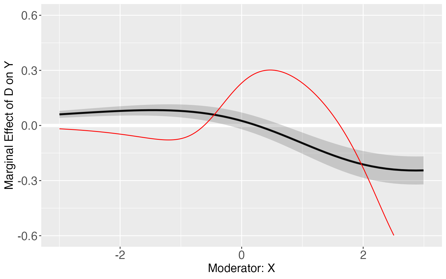
s8.linear$Avg.estimate
#> $`1`
#>                             ATE    sd z-value p-value lower CI(95%)
#> Average Treatment Effect -0.034 0.018  -1.889   0.059        -0.070
#>                          upper CI(95%)
#> Average Treatment Effect         0.001
In such cases, we can use the binning estimator as the diagnostic tools for the linear interaction effect (LIE) assumption, and use the kernel estimator to approximate the true DGP.
The binning estimator
The binning estimator is a diagnostic tool, it will discretizes the moderator X into several bins and create a dummy variable for each bin and picks an evaluation point within each bin, where users want to estimate the conditional marginal effect (CME) of on . The regression terms includes interactions between the bin dummies and the treatment indicator, the bin dummies and the moderator X minus the evaluation points, as well as the triple interactions.
If the CME estimates from the binning estimator sit closely to the estimated CME from the linear estimator, then the LIE assumption likely holds. For dataset s6, it is clear that all three binning estimators sits closely to the results from linear estimator.
s6.binning <- interflex(estimator = 'binning', data = s6, method='logit',
                        Y = 'Y', D = 'D', X = 'X',Z = c('Z1','Z2'))
plot(s6.binning)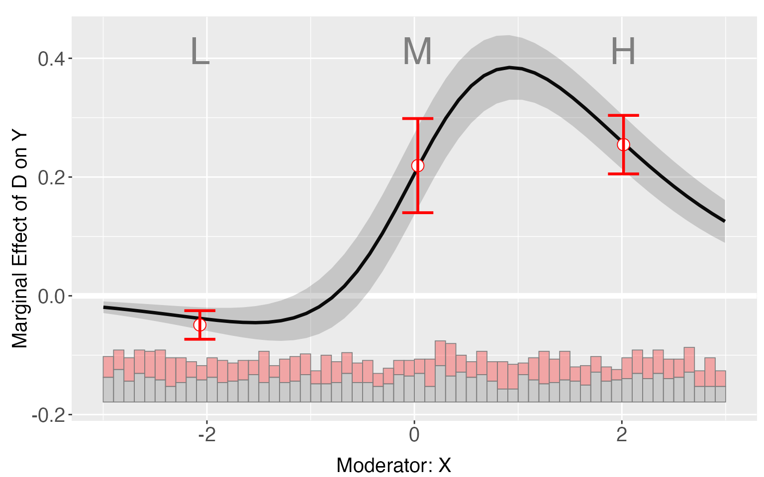
Users can access the estimated binning estimates saved in “est.bin”:
s6.binning$est.bin
#> $`1`
#>                         x0        coef         sd    CI.lower   CI.upper
#> X:[-3,-1.06]    -2.0681049 -0.04910873 0.01227520 -0.07318235 -0.0250351
#> X:(-1.06,0.971]  0.0328924  0.21922753 0.04043051  0.13993687  0.2985182
#> X:(0.971,2.99]   2.0159279  0.25455476 0.02512955  0.20527171  0.3038378
As a comparison, if we apply the binning method to s8, it is obvious that several binning estimates falls outside the confidence intervals of the linear estimates, implying the existence of non-linear predictor in the DGP of s8.
s8.binning <- interflex(estimator='binning', data = s8, method='logit',
                        Y = 'Y', D = 'D', X = 'X', Z = c('Z1','Z2'))
plot(s8.binning)
E(Y|X,D,Z)
Like the command for the linear estimator, one can visualize E(Y|X,D,Z) estimated using the binning model. It is expected to see some “zigzags” at the bin boundaries in the plot.
predict(s8.binning)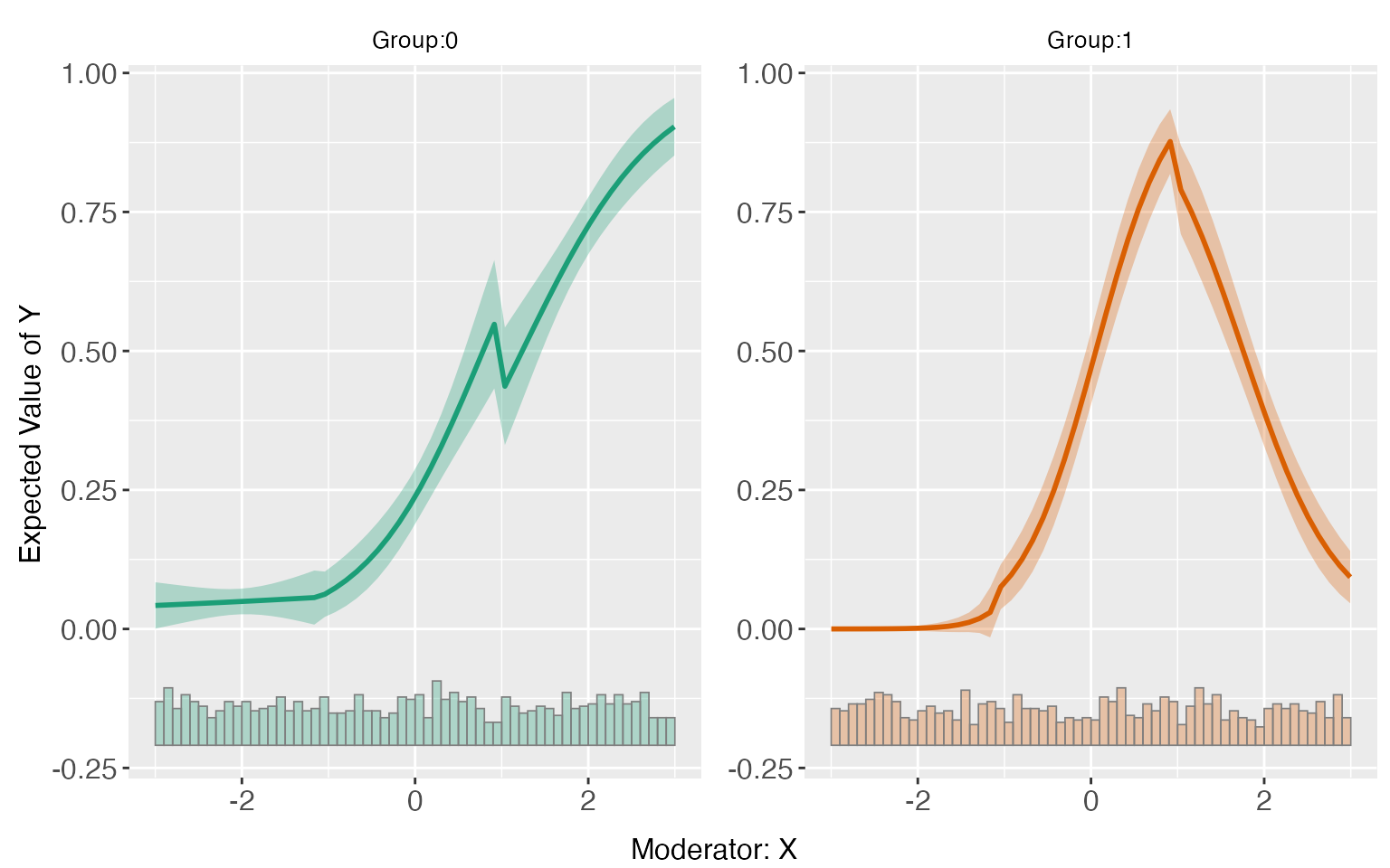
Hypothesis testing
The program provides formal tools for verifying the the LIE assumption, the Wald test and the likelihood ratio test. For dataset s8, both of these two tests reject the null hypothesis of LIE.
s8.binning$tests
#> $treat.type
#> [1] "discrete"
#>
#> $X.Lkurtosis
#> [1] "-0.002"
#>
#> $p.wald
#> [1] "0.000"
#>
#> $p.lr
#> [1] "0.000"
#>
#> $formula.restrict
#> Y ~ X + D.Group.2 + DX.Group.2 + Z1 + Z2
#> <environment: 0x13af937b0>
#>
#> $formula.full
#> Y ~ X + D.Group.2 + DX.Group.2 + Z1 + Z2 + G.2 + G.2.X + D.Group.2.G.2 +
#>     DX.Group.2.G.2 + G.3 + G.3.X + D.Group.2.G.3 + DX.Group.2.G.3
#> <environment: 0x13af937b0>
#>
#> $sub.test
#> NULL
For s6, there is no enough evidence to reject the null hypothesis.
s6.binning$tests
#> $treat.type
#> [1] "discrete"
#>
#> $X.Lkurtosis
#> [1] "-0.002"
#>
#> $p.wald
#> [1] "0.167"
#>
#> $p.lr
#> [1] "0.274"
#>
#> $formula.restrict
#> Y ~ X + D.Group.2 + DX.Group.2 + Z1 + Z2
#> <environment: 0x12be6bea8>
#>
#> $formula.full
#> Y ~ X + D.Group.2 + DX.Group.2 + Z1 + Z2 + G.2 + G.2.X + D.Group.2.G.2 +
#>     DX.Group.2.G.2 + G.3 + G.3.X + D.Group.2.G.3 + DX.Group.2.G.3
#> <environment: 0x12be6bea8>
#>
#> $sub.test
#> NULL
Fully moderated model
Unlike the fully moderated model in the linear estimator, for the binning estimator, this program interacts all covariates with the moderator X in the same way as the treatment variable D. That is to say, for each covariate, we includes interactions between it and the bin dummies and the triple interactions. It can reduce biases when the impact of some covariates to the outcome doesn’t take a linear form of “X”, but sometimes it will also render the estimates unstable when the number of covariates is large.
s8.binning.full <- interflex(estimator = 'binning', data=s8,
                             Y = 'Y', D = 'D', X = 'X', Z = c('Z1','Z2'),
                             method = 'logit', full.moderate=TRUE)
plot(s8.binning.full)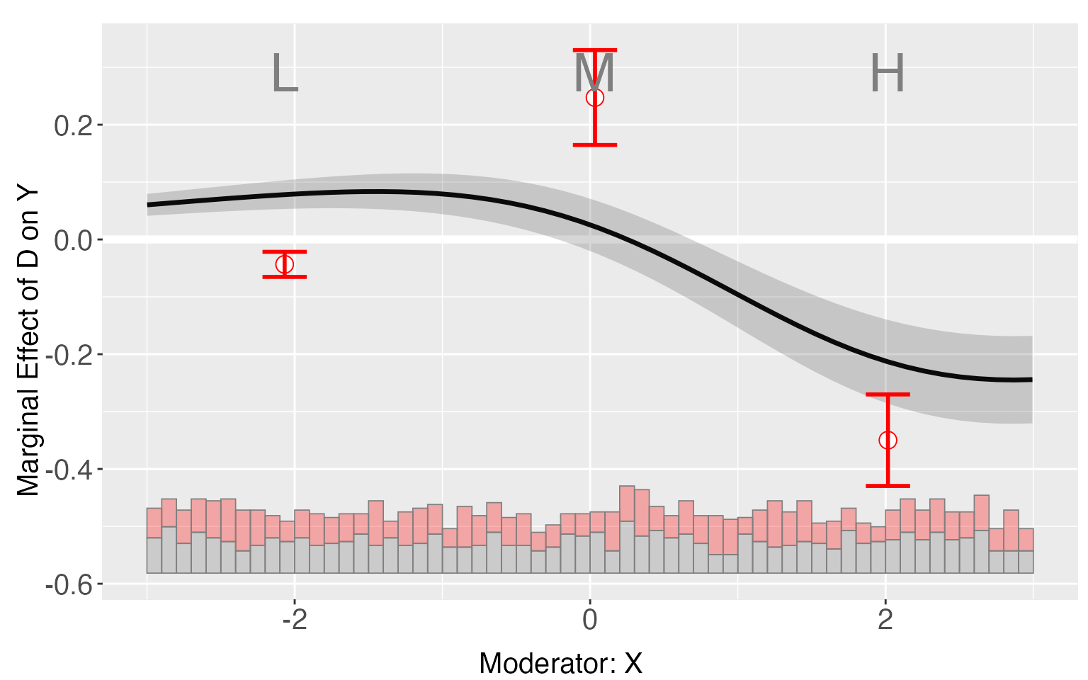
The kernel estimator
With the kernel method, a bandwidth is first selected via a 10-fold cross-validation. If the outcome variable is binary, the bandwidth that produces the largest area under the curve(AUC) or the least cross entropy in cross validation will be chosen as the “optimal” bandwidth. The standard errors are produced by a non-parametric bootstrap. It is very flexible but takes more time compared with the linear estimation.
For s8, the kernel estimator can much better approximates the “True” TE than the linear estimator.
s8.kernel <- interflex(estimator = 'kernel', data = s8, method='logit',
                       Y = 'Y', D = 'D', X = 'X', Z = c('Z1','Z2'),vartype = "bootstrap",
                      nboots = 1000, parallel = TRUE, cores = 31)
plot(s8.kernel)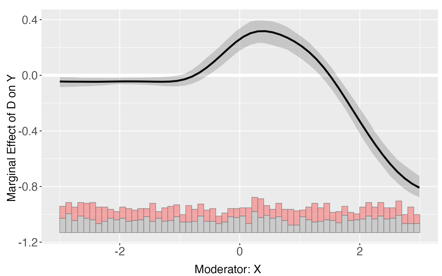
s8.kernel.plot <- plot.interflex(s8.kernel,show.all = T,Xdistr = 'none')$`1`
#link3 <- -1+d1+x+d1*x-d1*x*x
TE <- exp(-1+1+x+1*x-x*x)/(1+exp(-1+1+x+1*x-x*x))-exp(-1+0+x+0*x)/(1+exp(-1+0+x+0*x))
s8.kernel.plot + geom_line(aes(x=x,y=TE),color='red')+ylim(-0.6,0.6)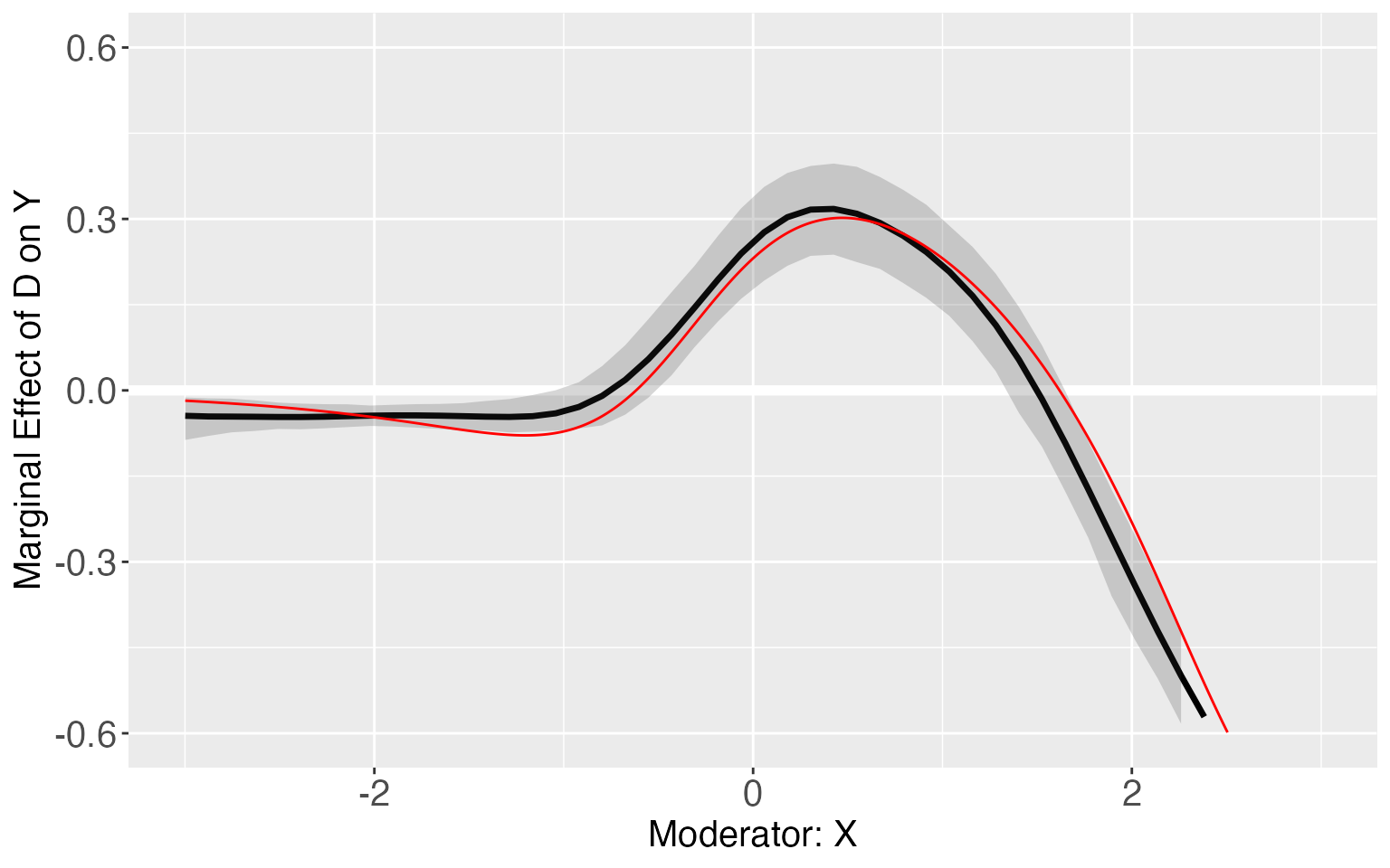
The results of cross-validation are saved in “CV.output”.
s8.kernel$CV.output
#>              bw Num.Eff.Points Cross Entropy       AUC       MSE       MAE
#>  [1,] 0.1198483             50     0.4256515 0.8718164 0.1346036 0.2602298
#>  [2,] 0.1371567             50     0.4205905 0.8728833 0.1341479 0.2604495
#>  [3,] 0.1569648             50     0.4170183 0.8736243 0.1337583 0.2606257
#>  [4,] 0.1796335             50     0.4145070 0.8744016 0.1334492 0.2608351
#>  [5,] 0.2055761             50     0.4126474 0.8751218 0.1332141 0.2611309
#>  [6,] 0.2352652             50     0.4112215 0.8756985 0.1330337 0.2615293
#>  [7,] 0.2692421             50     0.4101063 0.8759128 0.1328873 0.2620108
#>  [8,] 0.3081258             50     0.4092396 0.8761408 0.1327609 0.2625470
#>  [9,] 0.3526251             50     0.4085888 0.8765985 0.1326536 0.2631392
#> [10,] 0.4035510             50     0.4081388 0.8770013 0.1325803 0.2638362
#> [11,] 0.4618315             50     0.4079129 0.8771493 0.1325733 0.2647214
#> [12,] 0.5285289             50     0.4080061 0.8768740 0.1326836 0.2658942
#> [13,] 0.6048587             50     0.4085891 0.8762722 0.1329833 0.2674641
#> [14,] 0.6922120             50     0.4098780 0.8754857 0.1335652 0.2695497
#> [15,] 0.7921807             50     0.4120996 0.8744814 0.1345308 0.2722697
#> [16,] 0.9065869             50     0.4154569 0.8730803 0.1359699 0.2757136
#> [17,] 1.0375156             50     0.4200615 0.8702937 0.1379323 0.2798656
#> [18,] 1.1873528             50     0.4258355 0.8662769 0.1403815 0.2845302
#> [19,] 1.3588295             50     0.4324736 0.8606365 0.1431639 0.2893843
#> [20,] 1.5550707             50     0.4395246 0.8516951 0.1460492 0.2941300
#> [21,] 1.7796529             50     0.4465442 0.8393233 0.1488249 0.2985971
#> [22,] 2.0366691             50     0.4531849 0.8295647 0.1513576 0.3026954
#> [23,] 2.3308035             50     0.4592013 0.8230147 0.1535860 0.3063507
#> [24,] 2.6674165             50     0.4644548 0.8195111 0.1554944 0.3095131
#> [25,] 3.0526429             50     0.4689076 0.8173973 0.1570933 0.3121762
#> [26,] 3.4935034             50     0.4725954 0.8157592 0.1584092 0.3143708
#> [27,] 3.9980327             50     0.4755950 0.8147815 0.1594758 0.3161489
#> [28,] 4.5754258             50     0.4780007 0.8139460 0.1603300 0.3175705
#> [29,] 5.2362056             50     0.4799089 0.8134273 0.1610071 0.3186953
#> [30,] 5.9924147             50     0.4814095 0.8128858 0.1615394 0.3195781
For s6, the program will choose a relatively large bandwidth via cross-validation, thus the results produced by kernel estimator is similar to the results from the linear estimator.
s6.kernel <- interflex(estimator = 'kernel', data = s6, method = 'logit',
                       Y = 'Y',D = 'D', X = 'X',Z =c('Z1','Z2'),vartype = "bootstrap",
                      nboots = 1000, parallel = TRUE, cores = 31)
plot.interflex(s6.kernel)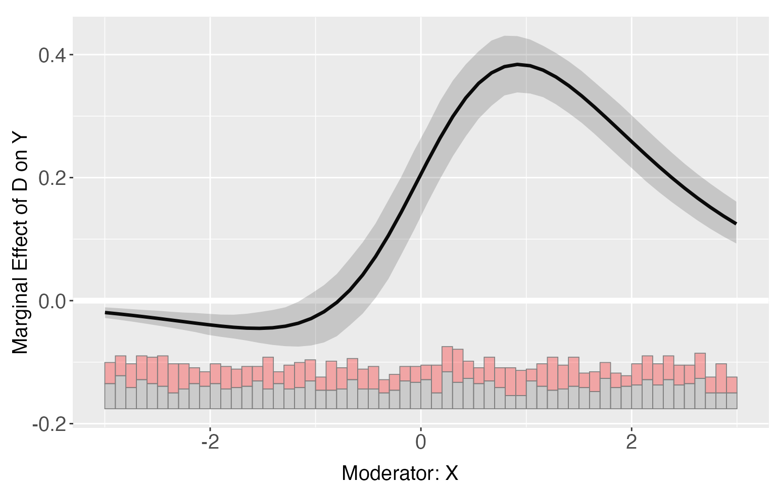
s6.kernel$CV.output
#>              bw Num.Eff.Points Cross Entropy       AUC       MSE       MAE
#>  [1,] 0.1198483             50     0.3790840 0.9096075 0.1194335 0.2290443
#>  [2,] 0.1371567             50     0.3765619 0.9098131 0.1190122 0.2294174
#>  [3,] 0.1569648             50     0.3745089 0.9101617 0.1186259 0.2296866
#>  [4,] 0.1796335             50     0.3726997 0.9102457 0.1182587 0.2298315
#>  [5,] 0.2055761             50     0.3710003 0.9105671 0.1179015 0.2298584
#>  [6,] 0.2352652             50     0.3693791 0.9111938 0.1175595 0.2298149
#>  [7,] 0.2692421             50     0.3678792 0.9117181 0.1172456 0.2297693
#>  [8,] 0.3081258             50     0.3665598 0.9119421 0.1169696 0.2297733
#>  [9,] 0.3526251             50     0.3654477 0.9125974 0.1167324 0.2298410
#> [10,] 0.4035510             50     0.3645313 0.9131210 0.1165284 0.2299518
#> [11,] 0.4618315             50     0.3637801 0.9138177 0.1163508 0.2300647
#> [12,] 0.5285289             50     0.3631667 0.9143141 0.1161962 0.2301347
#> [13,] 0.6048587             50     0.3626790 0.9146260 0.1160648 0.2301305
#> [14,] 0.6922120             50     0.3623139 0.9147510 0.1159563 0.2300512
#> [15,] 0.7921807             50     0.3620561 0.9149156 0.1158661 0.2299304
#> [16,] 0.9065869             50     0.3618677 0.9150078 0.1157867 0.2298120
#> [17,] 1.0375156             50     0.3617074 0.9151510 0.1157125 0.2297158
#> [18,] 1.1873528             50     0.3615545 0.9153893 0.1156421 0.2296309
#> [19,] 1.3588295             50     0.3614093 0.9154733 0.1155772 0.2295399
#> [20,] 1.5550707             50     0.3612787 0.9156498 0.1155200 0.2294381
#> [21,] 1.7796529             50     0.3611662 0.9157653 0.1154718 0.2293338
#> [22,] 2.0366691             50     0.3610721 0.9158573 0.1154325 0.2292375
#> [23,] 2.3308035             50     0.3609951 0.9159593 0.1154015 0.2291556
#> [24,] 2.6674165             50     0.3609332 0.9160753 0.1153775 0.2290895
#> [25,] 3.0526429             50     0.3608844 0.9160954 0.1153593 0.2290379
#> [26,] 3.4935034             50     0.3608464 0.9160856 0.1153456 0.2289983
#> [27,] 3.9980327             50     0.3608171 0.9160862 0.1153354 0.2289680
#> [28,] 4.5754258             50     0.3607948 0.9161170 0.1153278 0.2289450
#> [29,] 5.2362056             50     0.3607777 0.9161078 0.1153221 0.2289275
#> [30,] 5.9924147             50     0.3607647 0.9161185 0.1153178 0.2289143
E(Y|D,X,Z)
Like the linear estimator, the estimated conditional effects, , is saved in “pred.kernel”. Users can visualize it using the command “predict”.
predict(s8.kernel)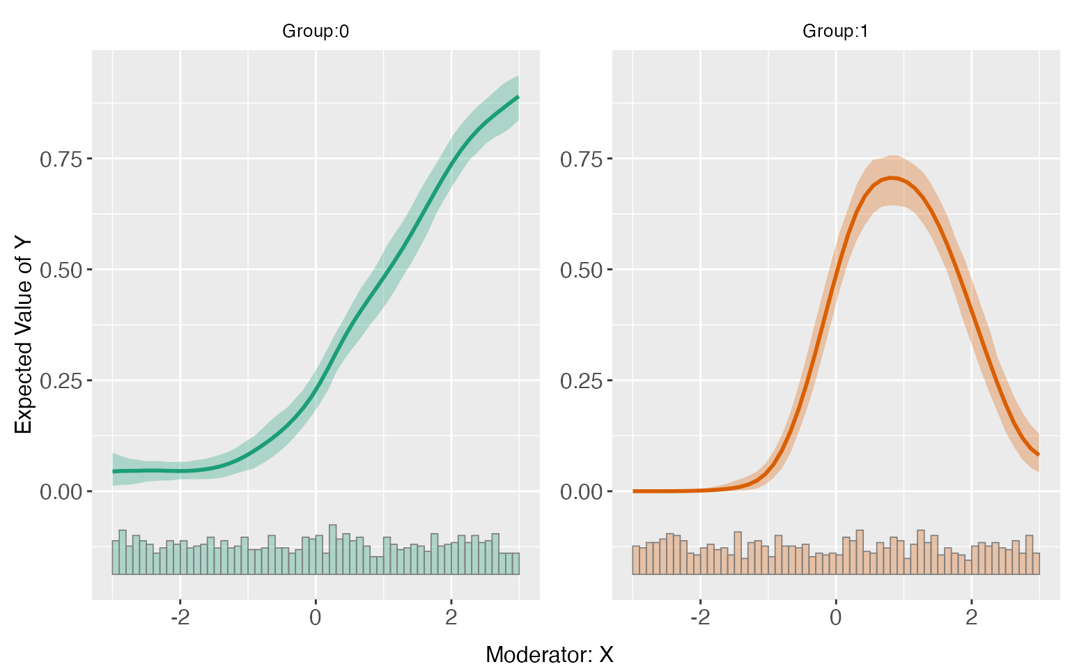
Differences in CME
Like the linear estimator, the estimated difference of treatment effects are saved in “diff.estimate”:
s8.kernel$diff.estimate
#> $`1`
#>            diff.estimate    sd z-value p-value lower CI(95%) upper CI(95%)
#> 50% vs 25%         0.315 0.045   6.973   0.000         0.221         0.399
#> 75% vs 50%        -0.242 0.058  -4.169   0.000        -0.363        -0.132
#> 75% vs 25%         0.073 0.045   1.629   0.103        -0.014         0.160
Average treatment effects
The estimated ATE for the kernel model is saved in “Avg.estimate”:
s8.kernel$Avg.estimate
#> $`1`
#>                             ATE    sd z-value p-value lower CI(95%)
#> Average Treatment Effect -0.055 0.019  -2.869   0.004        -0.090
#>                          upper CI(95%)
#> Average Treatment Effect        -0.017
fully moderated model
The fully moderated model for the kernel estimator adds the interaction terms between covariates and moderator to the local weighted regression.
s8.kernel.full <- interflex(estimator = 'kernel', data = s8, method='logit',
                            Y = 'Y',D = 'D', X = 'X', Z = c('Z1','Z2'),
                            full.moderate = TRUE,vartype = "bootstrap",
                            nboots = 1000, parallel = TRUE, cores = 31)
plot(s8.kernel.full)
Multiple (>2) treatment arms
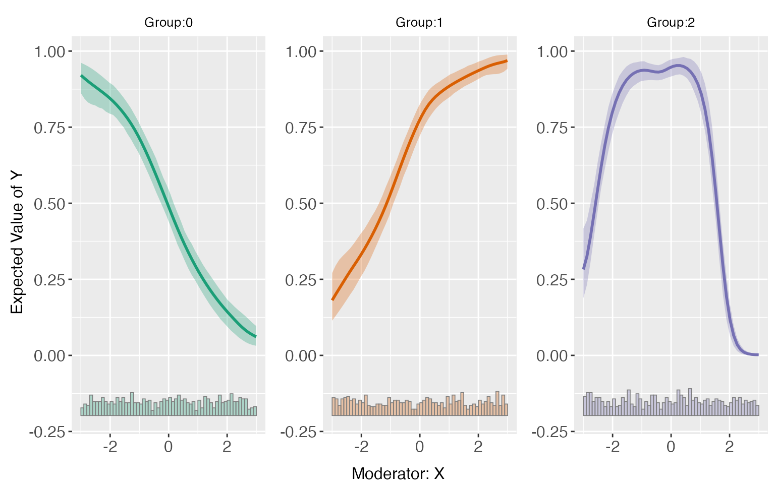
interflex can also be applied when there are more than two treated conditions. For s9, the LIE assumption are violated only in group 2. The linear estimator can give a consistent estimation of treatment effects for the group 1, but not group 2.
s9.linear <- interflex(estimator='linear', data=s9, method='logit',
                       Y = 'Y', D = 'D', X = 'X', Z = c('Z1','Z2'))
plot(s9.linear)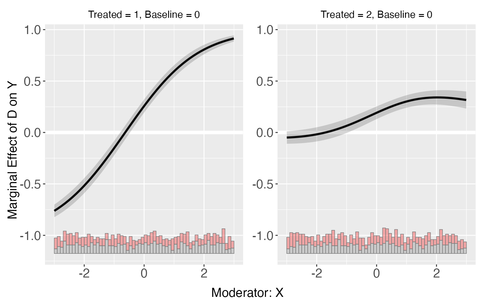
TE1 <- exp(1+x)/(1+exp(1+x))-exp(-x)/(1+exp(-x))
p1 <- plot.interflex(s9.linear,show.all = T)$`1`+geom_line(aes(x=x,y=TE1),color='red')
TE2 <- exp(4-x*x-x)/(1+exp(4-x*x-x))-exp(-x)/(1+exp(-x))
p2 <- plot(s9.linear,show.all = T)$`2`+geom_line(aes(x=x,y=TE2),color='red')
p1 + p2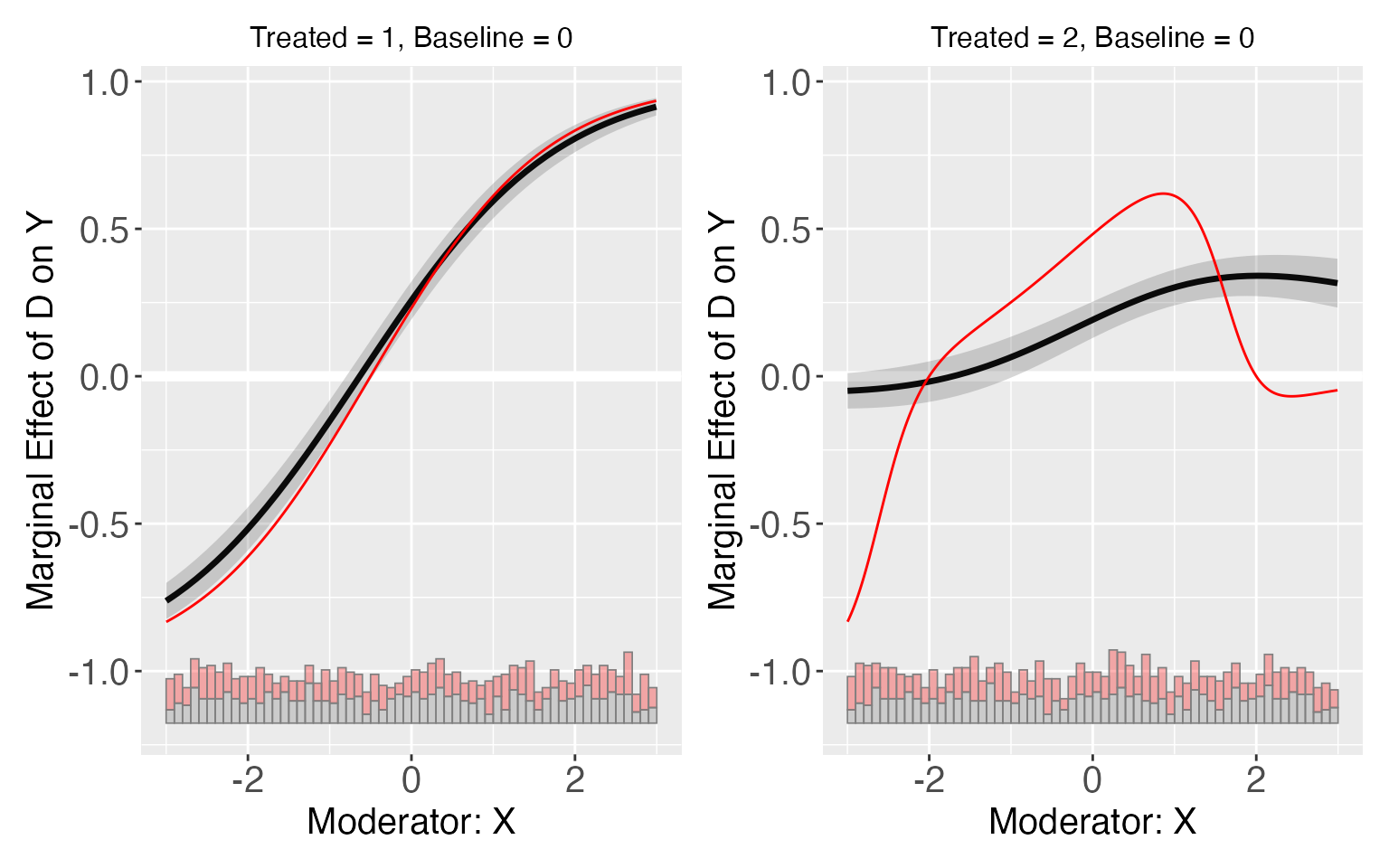
Then, we use the binning estimator to conduct a diagnostic analysis.
s9.binning <- interflex(estimator = 'binning', data = s9, method='logit',
                        Y = 'Y', D = 'D', X = 'X', Z = c('Z1','Z2'))
plot(s9.binning)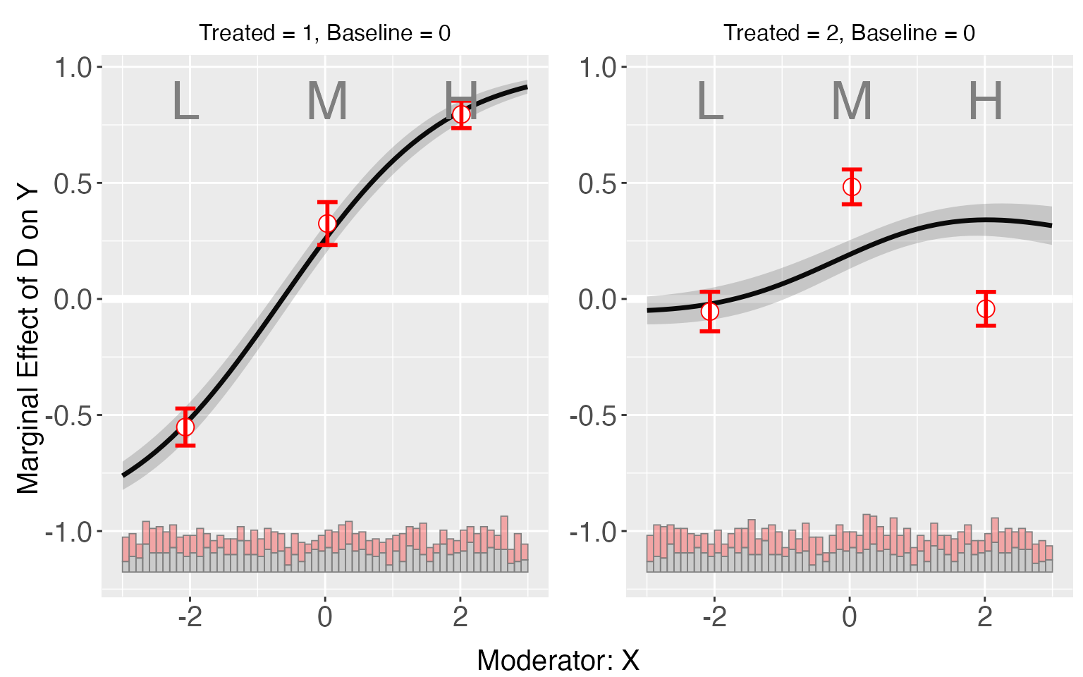
Results of the binning estimator also suggests the violation of LIE for group 2, which can be further verified by checking the test results.
s9.binning$tests$p.wald
#> [1] "0.000"
s9.binning$tests$p.lr
#> [1] "0.000"
Both of these tests suggest that LIE assumption fails in the model, but it doesn’t tell us in which group the assumption fails. There is an extra output “sub.test” when there are more than 3 groups in the data, which includes by-group results of the Wald/Likelihood ratio test, which test the linear multiplicative interaction assumption for each group. In this case, the test results suggest that there are not enough evidences to reject the null hypothesis for group 1, but for group 2, the null hypothesis can be safely rejected.
s9.binning$tests$sub.test
#> $`1`
#> $`1`$p.wald
#> [1] "0.195"
#>
#> $`1`$p.lr
#> [1] "0.193"
#>
#> $`1`$formula.restrict
#> Y ~ X + D.Group.2 + DX.Group.2 + D.Group.3 + DX.Group.3 + Z1 +
#>     Z2 + G.2 + G.2.X + D.Group.3.G.2 + DX.Group.3.G.2 + G.3 +
#>     G.3.X + D.Group.3.G.3 + DX.Group.3.G.3
#> <environment: 0x13b9436b0>
#>
#> $`1`$formula.full
#> Y ~ X + D.Group.2 + DX.Group.2 + D.Group.3 + DX.Group.3 + Z1 +
#>     Z2 + G.2 + G.2.X + D.Group.2.G.2 + DX.Group.2.G.2 + D.Group.3.G.2 +
#>     DX.Group.3.G.2 + G.3 + G.3.X + D.Group.2.G.3 + DX.Group.2.G.3 +
#>     D.Group.3.G.3 + DX.Group.3.G.3
#> <environment: 0x13b9436b0>
#>
#>
#> $`2`
#> $`2`$p.wald
#> [1] "0.000"
#>
#> $`2`$p.lr
#> [1] "0.000"
#>
#> $`2`$formula.restrict
#> Y ~ X + D.Group.2 + DX.Group.2 + D.Group.3 + DX.Group.3 + Z1 +
#>     Z2 + G.2 + G.2.X + D.Group.2.G.2 + DX.Group.2.G.2 + G.3 +
#>     G.3.X + D.Group.2.G.3 + DX.Group.2.G.3
#> <environment: 0x13b9436b0>
#>
#> $`2`$formula.full
#> Y ~ X + D.Group.2 + DX.Group.2 + D.Group.3 + DX.Group.3 + Z1 +
#>     Z2 + G.2 + G.2.X + D.Group.2.G.2 + DX.Group.2.G.2 + D.Group.3.G.2 +
#>     DX.Group.3.G.2 + G.3 + G.3.X + D.Group.2.G.3 + DX.Group.2.G.3 +
#>     D.Group.3.G.3 + DX.Group.3.G.3
#> <environment: 0x13b9436b0>
Lastly, we can use the kernel estimator to get more consistent results.
s9.kernel <- interflex(estimator = 'kernel', data = s9,
                       Y ='Y', D = 'D', X = 'X', Z = c('Z1','Z2'),
                       method='logit',vartype = "bootstrap",
                      nboots = 1000, parallel = TRUE, cores = 31)
plot(s9.kernel)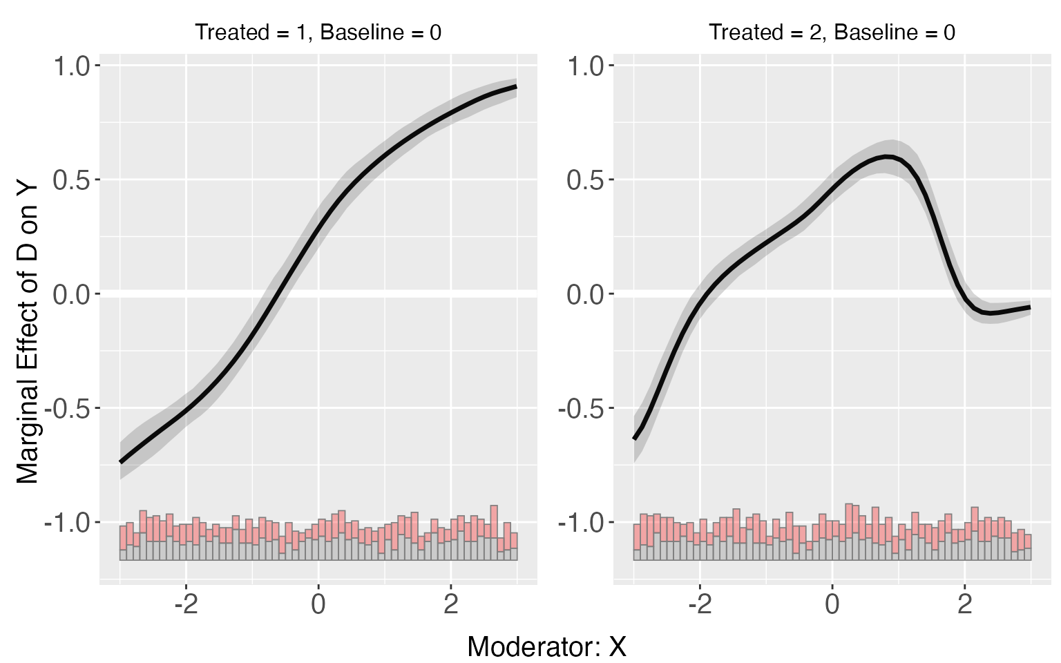
TE1 <- exp(1+x)/(1+exp(1+x))-exp(-x)/(1+exp(-x))
p1 <- plot(s9.kernel,show.all = T)$`1`+geom_line(aes(x=x,y=TE1),color='red')
TE2 <- exp(4-x*x-x)/(1+exp(4-x*x-x))-exp(-x)/(1+exp(-x))
p2 <- plot(s9.kernel,show.all = T)$`2`+geom_line(aes(x=x,y=TE2),color='red')
p1 + p2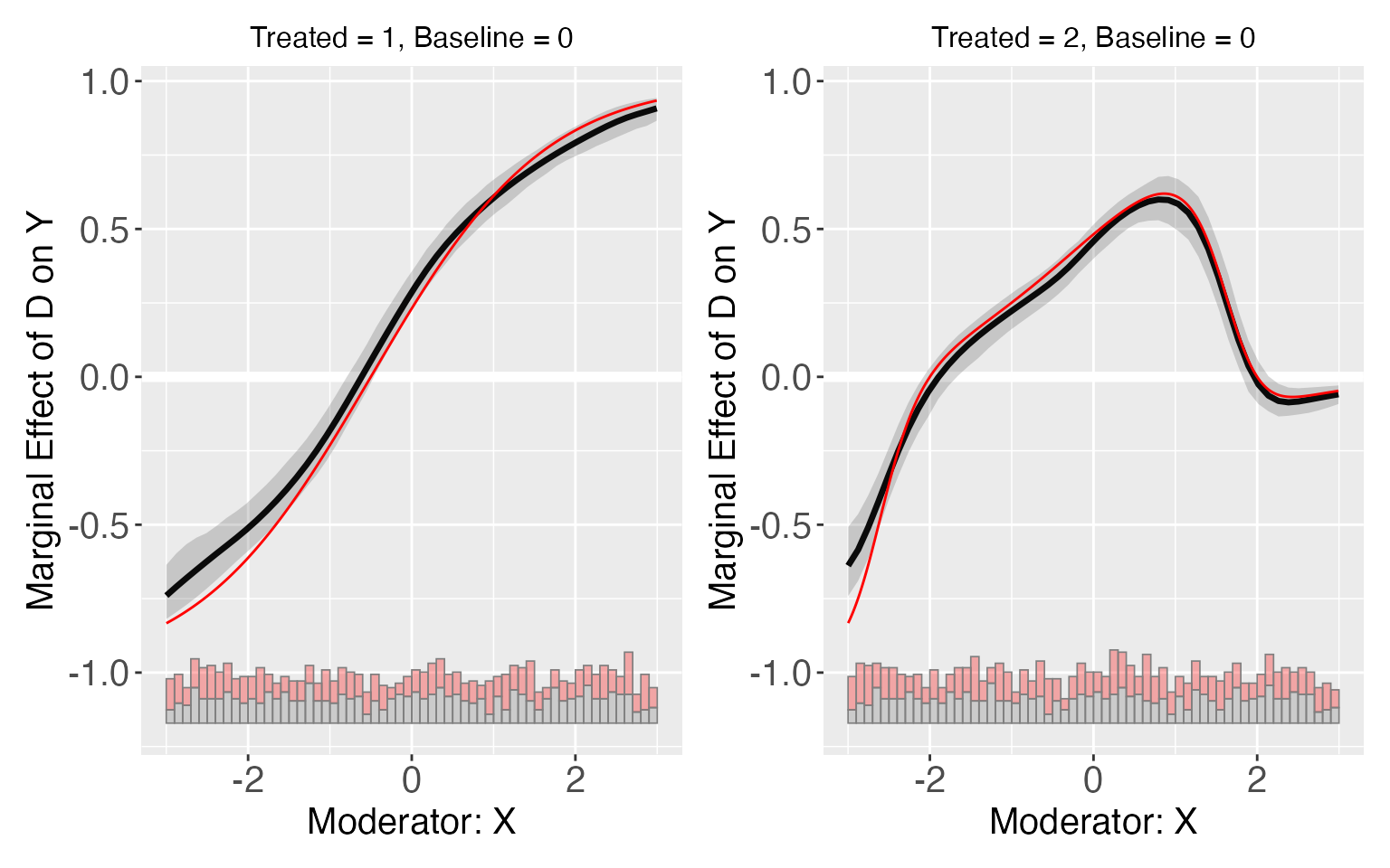
The estimated ATE and E(Y|D,X,Z) are also grouped by treatment.
s9.kernel$Avg.estimate
#> $`1`
#>                            ATE    sd z-value p-value lower CI(95%)
#> Average Treatment Effect 0.175 0.032   5.508   0.000         0.112
#>                          upper CI(95%)
#> Average Treatment Effect         0.239
#>
#> $`2`
#>                            ATE    sd z-value p-value lower CI(95%)
#> Average Treatment Effect 0.153 0.025   6.188   0.000         0.104
#>                          upper CI(95%)
#> Average Treatment Effect         0.201
predict(s9.kernel)