Interflex with Continuous Outcomes • interflex

Let’s load the package as well as the simulated toy datasets. Note that s6-s9 are for the tutorial for interflex with discrete outcomes.

library(interflex)
data(interflex)
ls()
#>  [1] "app_hma2015"    "app_vernby2013" "s1"             "s2"            
#>  [5] "s3"             "s4"             "s5"             "s6"            
#>  [9] "s7"             "s8"             "s9"

s1 is a case of a dichotomous treatment indicator with linear marginal effects; s2 is a case of a continuous treatment indicator with linear marginal effects; s3 is a case of a dichotomous treatment indicator with nonlinear marginal effects; s4 is a case of a dichotomous treatment indicator, nonlinear marginal effects, with additive two-way fixed effects; and s5 is a case of a discrete treatment indicator, nonlinear marginal effects, with additive two-way fixed effects. s1-s5 are generated using the following code:

set.seed(1234)
n<-200
d1<-sample(c(0,1),n,replace=TRUE) # dichotomous treatment
d2<-rnorm(n,3,1) # continuous treatment
x<-rnorm(n,3,1) # moderator
z<-rnorm(n,3,1) # covariate
e<-rnorm(n,0,1) # error term

## linear marginal effect
y1<-5 - 4 * x - 9 * d1 + 3 * x * d1 + 1 * z + 2 * e
y2<-5 - 4 * x - 9 * d2 + 3 * x * d2 + 1 * z + 2 * e
s1<-cbind.data.frame(Y = y1, D = d1, X = x, Z1 = z)
s2<-cbind.data.frame(Y = y2, D = d2, X = x, Z1 = z)

## quadratic marginal effect
x3 <- runif(n, -3,3) # uniformly distributed moderator
y3 <- d1*(x3^2-2.5) + (1-d1)*(-1*x3^2+2.5) + 1 * z + 2 * e
s3 <- cbind.data.frame(D=d1, X=x3, Y=y3, Z1 = z)

## adding two-way fixed effects
n  <- 500
d4 <-sample(c(0,1),n,replace=TRUE) # dichotomous treatment
x4 <- runif(n, -3,3) # uniformly distributed moderator
z4 <- rnorm(n, 3,1) # covariate
alpha <- 20 * rep(rnorm(n/10), each = 10)
xi <- rep(rnorm(10), n/10)
y4 <- d4*(x4^2-2.5) + (1-d4)*(-1*x4^2+2.5) + 1 * z4 + 
  alpha + xi + 2 * rnorm(n,0,1)
s4 <- cbind.data.frame(D=d4, X=x4, Y=y4, Z1 = z4, unit = rep(1:(n/10), each = 10), year = rep(1:10, (n/10)))

## Multiple treatment arms
n <- 600
# treatment 1
d1 <- sample(c('A','B','C'),n,replace=T)
# moderator
x <- runif(n,min=-3, max = 3)
# covriates
z1 <- rnorm(n,0,3)
z2 <- rnorm(n,0,2)
# error
e <- rnorm(n,0,1)
y1 <- rep(NA,n)
y1[which(d1=='A')] <- -x[which(d1=='A')]
y1[which(d1=='B')] <- (1+x)[which(d1=='B')]
y1[which(d1=='C')] <- (4-x*x-x)[which(d1=='C')]
y1 <- y1 + e + z1 + z2
s5 <- cbind.data.frame(D=d1, X=x, Y=y1, Z1 = z1,Z2 = z2)

The implied population marginal effects for the DGPs of s1 and s2 are \[ME(X) = 3X - 9;\] the implied population marginal effects for the DGPs of s3 and s4 are \[ME(X) = 2X^{2} - 5.\] For s5, if we set treatment “A” as our base category, the implied population marginal effects for group “B” and group “C” are, respectively, \[ME(X) = 2X + 1\quad\text{and}\quad ME(X) = -X^{2} + 4.\]

The interflex package ships the following functions: interflex, inter.raw, inter.gam, plot. The functionalities of inter.binning and inter.kernel covered by interflex, but they are still supported for backward compatibility.

Raw plots

The first step of the diagnostics is to plot raw data. We supply the function interflex with the variable names of the outcome Y, the treatment D, and the moderator X. You can also supply labels for these variables. If you supply a variable name to the weights option, the linear and LOESS fits will be adjusted based on the weights. Note that the correlations between covariates Z and Y are NOT partialed out. We use main to add a title to the plot and cex.main to adjust its size.

interflex(estimator = "raw",Y = "Y", D = "D", X = "X", data = s1, 
          weights = NULL, Ylabel = "Outcome", 
          Dlabel = "Treatment", Xlabel="Moderator", 
          main = "Raw Plot", cex.main = 1.2, ncols=2)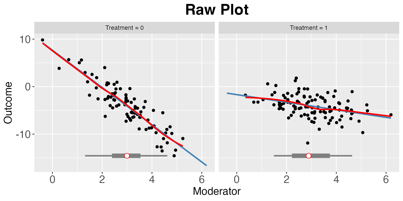

A black-white theme is applied when we set theme.bw = TRUE. show.grid = FALSE can be used to remove grid in the plot. Both options are allowed in interflex and plot.

interflex(estimator = "raw", Y = "Y", D = "D", X = "X", data = s2, 
          Ylabel = "Outcome", Dlabel = "Treatment", Xlabel="Moderator", 
          theme.bw = TRUE, show.grid = FALSE, ncols=3)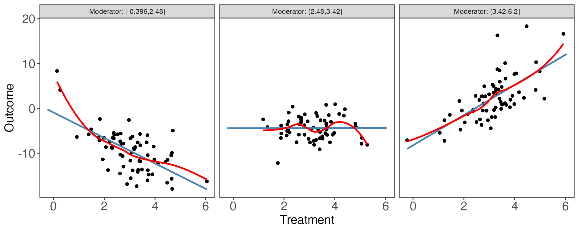

interflex(estimator = "raw", Y = "Y", D = "D", X = "X", data = s3, 
          Ylabel = "Outcome", Dlabel = "Treatment", Xlabel="Moderator",
          ncols=3)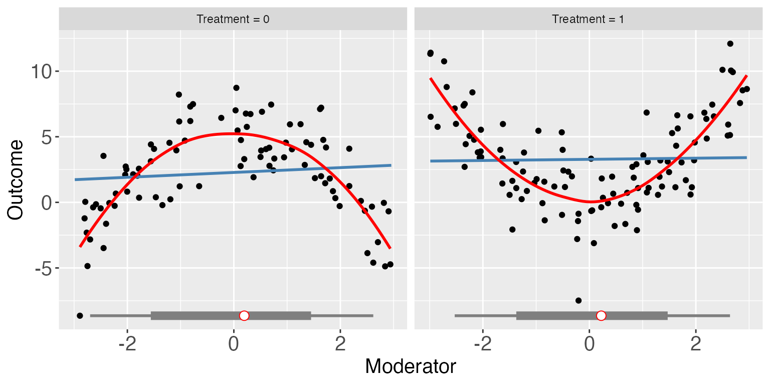

For the continuous treatment case (e.g. s2), we can also draw a Generalized Additive Model (GAM) plot. You can supply a set of covariates to be controlled for by supplying Z, which takes a vector of covariate names (strings).

interflex(estimator = "gam",Y="Y", D="D", X="X", Z=c("Z1"), data=s2)

#> 
#> Family: gaussian 
#> Link function: identity 
#> 
#> Formula:
#> Y ~ s(D, X, k = 10) + Z1
#> 
#> Estimated degrees of freedom:
#> 8.85  total = 10.85 
#> 
#> GCV score: 4.59025

The binning estimator

The second diagnostic tool is the binning plot. The nbins option sets the number of bins. The default number of bins is 3, and equal-sized bins are created based on the distribution of the moderator. There are four options for the choice of the vcov estimator: vcov.type = "homoscedastic", "robust", "cluster",and "pcse". The default option is "robust".

Note that interflex will also automatically report a set of statistics when estimator = "binning", including: (1) the binning estimates and their standard errors and 95% confidence intervals, (2) the percentage of observations within each bin, (3) the L-kurtosis of the moderator, and (4) a Wald test to formally test if we can reject the linear multiplicative interaction model by comparing it with a more flexible model of multiple bins. .

out <- interflex(Y = "Y", D = "D", X = "X", Z = "Z1", data = s1, 
                 estimator = "binning", vcov.type = "robust", 
                 main = "Marginal Effects", ylim = c(-15, 15))
#> Baseline group not specified; choose treat = 0 as the baseline group.
plot(out)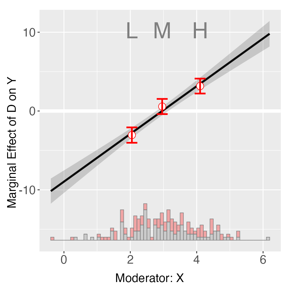

print(out$tests$p.wald)
#> [1] "0.582"

We see that the Wald test cannot reject the NULL hypothesis that the linear interaction model and the three-bin model are statistically equivalent. If we only want to conduct the linear estimator, we can set estimator = "linear", We also report the uniform/simultaneous confidence interval (when setting vartype = "bootstrap"), as depicted by the dashed lines.

out2 <- interflex(Y = "Y", D = "D", X = "X", Z = "Z1", data = s1, 
                  estimator = "linear", vcov.type = "robust", 
                  main = "Marginal Effects", ylim = c(-15, 15))
#> Baseline group not specified; choose treat = 0 as the baseline group.
plot(out2)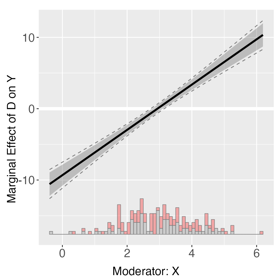

You can access estimates, as well as pointwise and uniform confidence intervals, from est.lin.

head(out2$est.lin$`1`)
#>                 X         ME        sd lower CI(95%) upper CI(95%)
#> [1,] -0.396063535 -10.575601 0.8349589    -12.222311     -8.928892
#> [2,] -0.261533642 -10.148629 0.8046173    -11.735499     -8.561760
#> [3,] -0.127003750  -9.721657 0.7744186    -11.248969     -8.194346
#> [4,]  0.007526143  -9.294685 0.7443803    -10.762755     -7.826616
#> [5,]  0.142056035  -8.867713 0.7145225    -10.276898     -7.458529
#> [6,]  0.276585928  -8.440741 0.6848689     -9.791443     -7.090040
#>      lower uniform CI(95%) upper uniform CI(95%)
#> [1,]             -12.61342             -8.537779
#> [2,]             -12.11240             -8.184860
#> [3,]             -11.61172             -7.831592
#> [4,]             -11.11144             -7.477932
#> [5,]             -10.61160             -7.123832
#> [6,]             -10.11225             -6.769233

plot allows users to adjust graphic options without re-estimating the model. The first entry must be a interflex object. Note that we use bin.labs = FALSE to hide the label on the top of each bin and Xdistr = "none" to remove the distribution of the moderator (not recommended). We use cex.axis and cex.lab to adjust the font sizes of axis numbers and labels.

plot(out, xlab = "Moderate is X", Xdistr = "none", bin.labs = FALSE, cex.axis = 0.8, cex.lab = 0.8)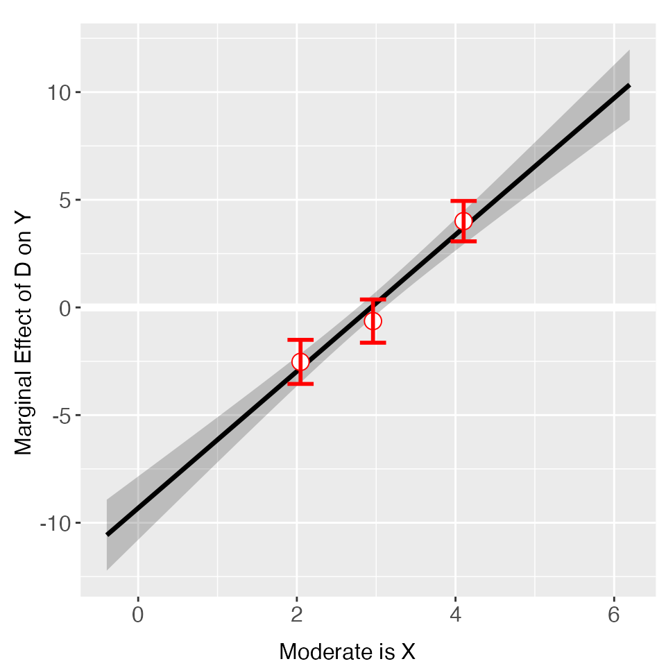

Next, we use Xunif = TRUE to transform the moderator into a uniformly distributed random variable (based on the rank order in values of the orginal moderator) before estimating the marginal effects. nbins = 4 sets the number of bins to 4.

out <- interflex(Y = "Y", D = "D", X = "X", Z = "Z1", data = s1, 
                 estimator = "binning", nbins = 4, 
                 theme.bw = TRUE, Xunif = TRUE)
#> Baseline group not specified; choose treat = 0 as the baseline group.
out$figure

The binning estimates for the continuous case are shown below. We now present the distribution of the moderator with a density plot using option Xdist = "density" – the default option is "hist" or "histogram". We turn off the bin labels using bin.labs = FALSE.

out <- interflex(Y = "Y", D = "D", X = "X", Z = "Z1", data = s2, 
                 estimator = "binning", Xdistr = "density", 
                 bin.labs = FALSE)
out$figure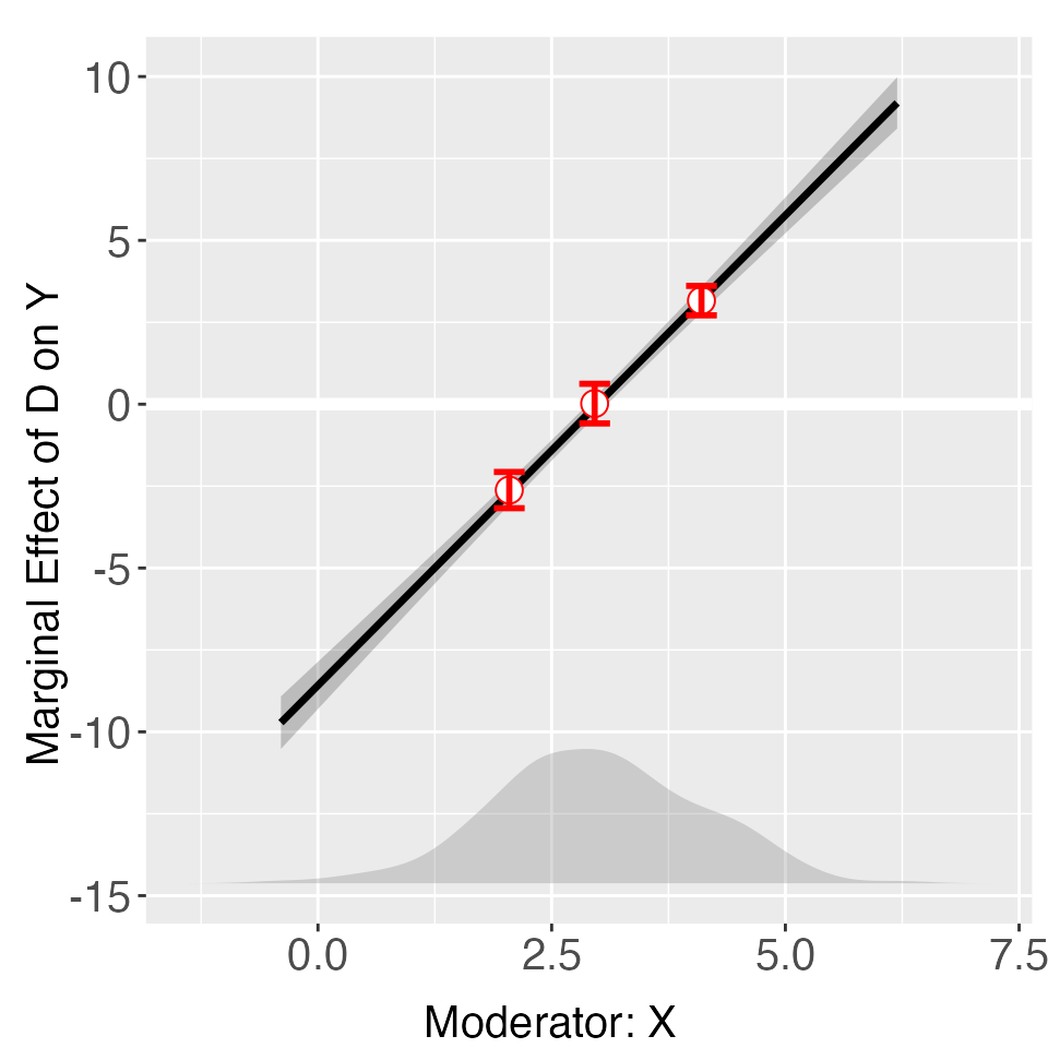

Note that you can customize the cutoff values for the bins, for example, set cutoffs = c(1, 2, 4, 5) to create five bins: [minX, 1], (1, 2], (2,4], (4, 5] and (5,maxX] (supplying N numbers will create N+1 bins). Note that the cutoffs option will override the nbins option if they are incompatible.

out <- interflex(Y = "Y", D = "D", X = "X", Z = "Z1", data = s2, 
                 estimator = "binning", cutoffs = c(1,2,4,5))
out$figure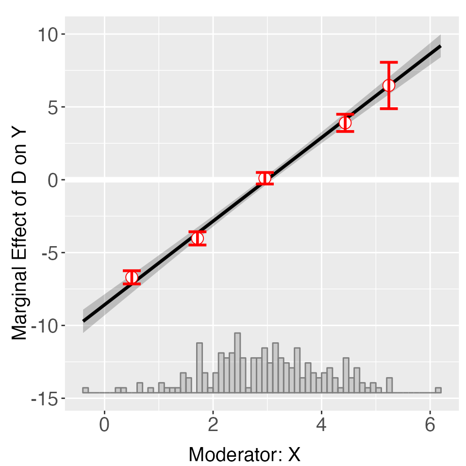

The binning estimates for the dichotomous, nonlinear case (i.e. s3) are shown below. A linear interaction model clearly gives misleading marginal effects estimates. The marginal effects plot is stored in out$figure while the estimates and standard errors are stored in out$est.linear (linear) and out$est.bin (binning). The tests results are stored in out$tests (binning).

out <- interflex(Y = "Y", D = "D", X = "X", Z = "Z1", data = s3, 
                 estimator = "binning")
#> Baseline group not specified; choose treat = 0 as the baseline group.
print(out$tests$p.wald)
#> [1] "0.000"

This time the NULL hypothesis that the linear interaction model and the three-bin model are statistically equivalent is safely rejected (p.wald = 0.00).

The kernel estimator

With the kernel method, a bandwidth is first selected via 10-fold least-squares cross-validation.

The standard errors are produced by a non-parametric bootstrap (you can adjust the number of bootstrap iterations using the nboots option). The grid option can either be an integer, which specifies the number of bandwidths to be cross-validated, or a vector of candidate bandwidths – the default is grid = 20. You can also specify a clustered group structure by using the cl option, in which case a block bootstrap procedure will be performed.

Starting from v.1.1.0, we introduce adaptive bandwidth selection to interflex. This means that the bandwidth will be smaller in regions where there are more data and larger in regions where there are few data points (based on the moderator). When adaptive bandwidth is being used, bw refers to the bandwidth applied in the region with the highest density of observations.

Even with an optimized algorithm, the bootstrap procedure for large datasets can be slow. We incorporate parallel computing (parallel=TRUE) to speed it up. You can choose the number of cores to be used for parallel computing; otherwise the program will detect the number of logical cores in your computer and use as many cores as possible (warning: this will significantly slow down your computer!).

out <- interflex(Y = "Y", D = "D", X = "X", Z = "Z1", data = s1, vartype = 'bootstrap',
                 estimator = "kernel", nboots = 1000, 
                 parallel = TRUE, cores = 31)
#> Baseline group not specified; choose treat = 0 as the baseline group. 
#> Cross-validating bandwidth ... 
#> Parallel computing with 20 cores...
#> Optimal bw=6.592.
#> Number of evaluation points:50
#> Parallel computing with 20 cores...
#> 
out$figure

You can access estimates, as well as pointwise and uniform confidence intervals, from est.kernel.

head(out$est.kernel$`1`)
#>                 X         TE        sd lower CI(95%) upper CI(95%)
#> [1,] -0.396063535 -10.571474 0.8345364    -12.271839     -9.047824
#> [2,] -0.261533642 -10.144601 0.8042232    -11.770410     -8.679840
#> [3,] -0.127003750  -9.717700 0.7740682    -11.283608     -8.305695
#> [4,]  0.007526143  -9.290719 0.7440621    -10.806015     -7.941442
#> [5,]  0.142056035  -8.863690 0.7142049    -10.324891     -7.567790
#> [6,]  0.276585928  -8.436683 0.6845219     -9.839558     -7.194474
#>      lower uniform CI(95%) upper uniform CI(95%)
#> [1,]             -12.68872             -8.442099
#> [2,]             -12.20087             -8.102324
#> [3,]             -11.71434             -7.754390
#> [4,]             -11.22775             -7.390994
#> [5,]             -10.74093             -7.027841
#> [6,]             -10.25380             -6.679131

If you specify a bandwidth manually (for example, by setting bw = 1), the cross-validation step will be skipped. The main option controls the title of the plot while the xlim and ylim options control the ranges of the x-axis and y-axis, respectively.

out <- interflex(Y = "Y", D = "D", X = "X", Z = "Z1", data = s1, 
       estimator = "kernel", nboots = 1000, bw = 1, 
       main = "The Linear Case", parallel = TRUE, cores = 31,vartype = 'bootstrap',
       xlim = c(-0.5,6.5), ylim = c(-15, 15))
out$figure

For dataset s3, the kernel method produces non-linear marginal effects estimates that are much closer to the effects implied by the true DGP.

out <- interflex(Y = "Y", D = "D", X = "X", Z = "Z1", data = s3, vartype = 'bootstrap',
                 estimator = "kernel", theme.bw = TRUE, nboots = 1000, parallel = TRUE, cores = 31)
out$figure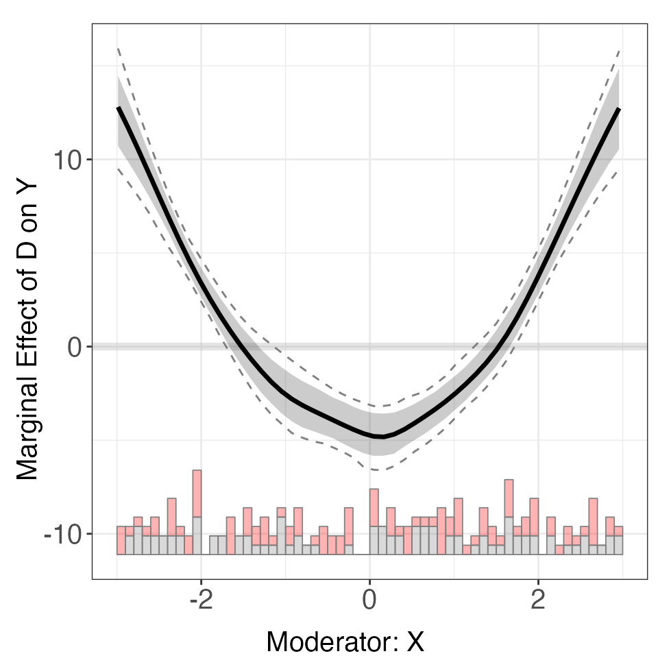

Again, if we only want to change the look of a marginal effect plot, we can use plot to save time. CI = FALSE removes the confidence interval ribbon.

plot(out, main = "Nonlinear Marginal Effects", 
     ylab = "Coefficients", Xdistr = "density", 
     xlim = c(-3,3), ylim = c(-10,12), CI = FALSE, 
     cex.main = 0.8, cex.lab = 0.7, cex.axis = 0.7)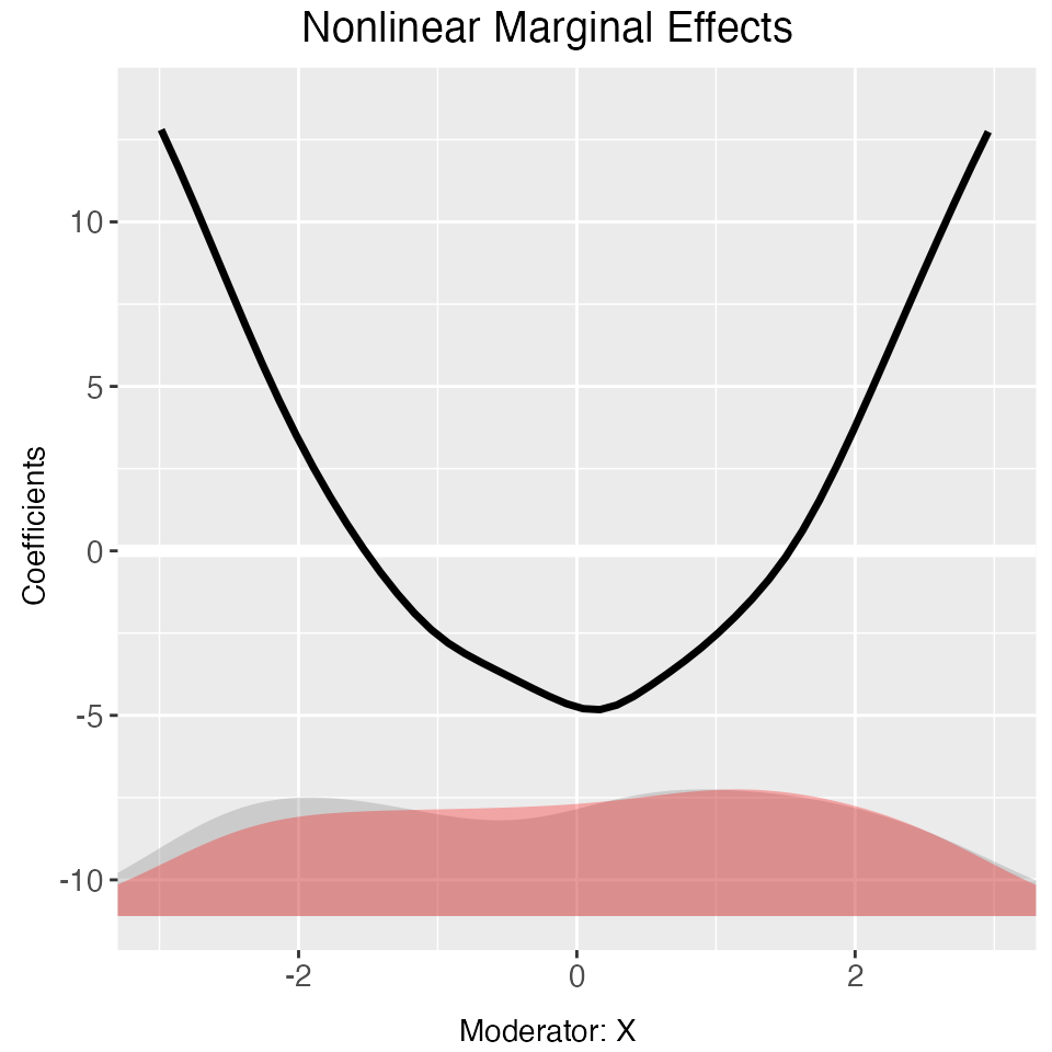

The semi-parametric marginal effect estimates are stored in out$est.kernel.

Note that we can use the file option to save a plot to a file in interflex (e.g. by setting file = "myplot.pdf" or file = "myplot.png").

Fixed effects

We move on to linear fixed effects models. Remember in s4, a large chunk of the variation in the outcome variable is driven by group fixed effects. Below is a scatterplot of the raw data (group index vs. outcome). Red and green dots represent treatment and control units, respectively. We can see that outcomes are highly correlated within a group.

library(ggplot2)
ggplot() + geom_point(data = s4,aes(x = unit, y = Y, colour = as.factor(D))) + 
  guides(colour=FALSE)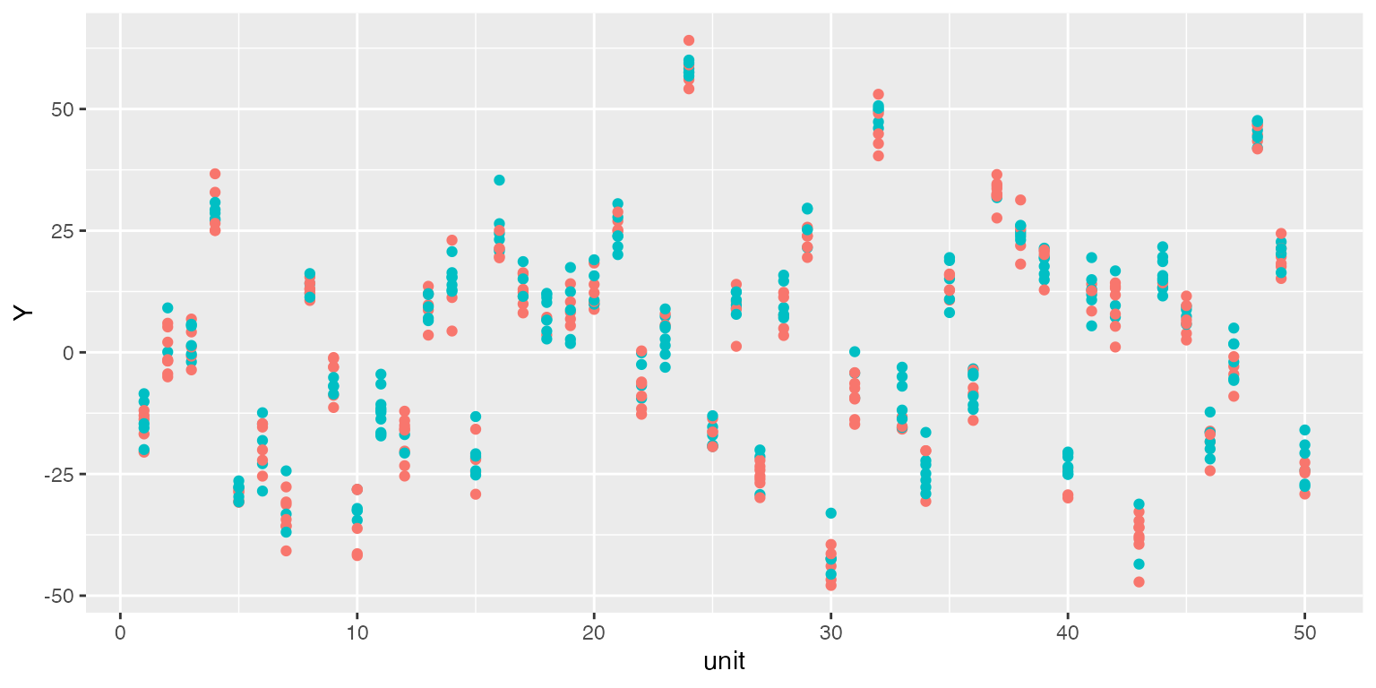

When fixed effects are present, it is possible that we cannot observe a clear pattern of marginal effects in the raw plot as before, while binning estimates have wide confidence intervals:

interflex(estimator = "raw", Y = "Y", D = "D", X = "X", data = s4, 
          weights = NULL,ncols=2)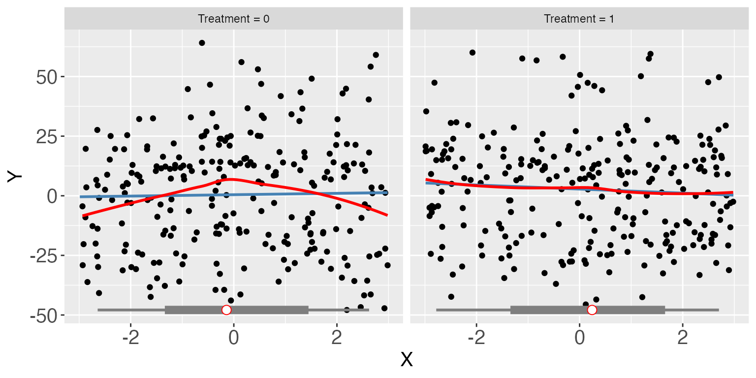

s4.binning <- interflex(Y = "Y", D = "D", X = "X", Z = "Z1", data = s4, 
                        estimator = "binning", FE = NULL, cl = "unit")
plot(s4.binning)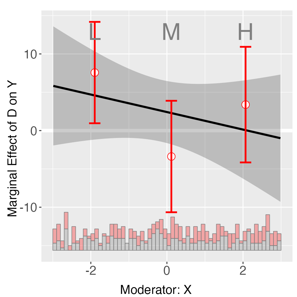

The binning estimates are much more informative when fixed effects are included, by using the FE option. Note that the number of group indicators can exceed 2. Our algorithm is optimized for a large number of fixed effects or many group indicators. The cl option controls the level at which standard errors are clustered.

s4$wgt <- 1
s4.binning <- interflex(Y = "Y", D = "D", X = "X", Z = "Z1", data = s4, 
                        estimator = "binning", FE = c("unit", "year"), 
                        cl = "unit", weights = "wgt")
plot(s4.binning)

When fixed effects are not taken into account, the kernel estimates are also less precisely estimated. Because the model is incorrectly specified, cross-validated bandwidths also tend to be bigger than optimal.

s4.kernel <- interflex(Y = "Y", D = "D", X = "X", Z = "Z1", data = s4, 
                       estimator = "kernel", FE = NULL, vartype = 'bootstrap',
                       nboots = 1000, parallel = TRUE, cores = 31,
                       cl = "unit", weights = "wgt")
plot(s4.kernel)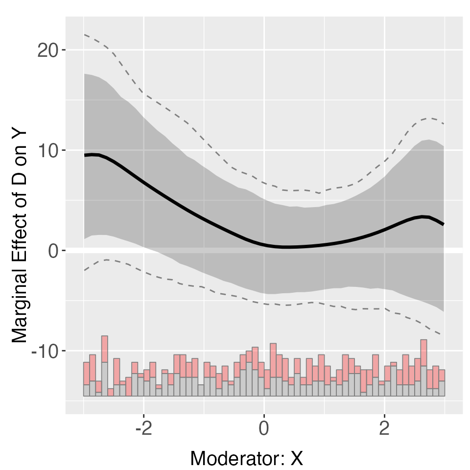

Controlling for fixed effects by using the FE option solves this problem. The estimates are now much closer to the population truth. Note that all uncertainty estimates are produced via bootstrapping. When the cl option is specified, a block bootstrap procedure will be performed.

s4.kernel <- interflex(Y = "Y", D = "D", X = "X", Z = "Z1", data = s4, 
                       estimator = "kernel", FE = c("unit","year"), cl = "unit",vartype = 'bootstrap',
                       nboots = 1000, parallel = TRUE, cores = 31,weights = "wgt")
plot(s4.kernel)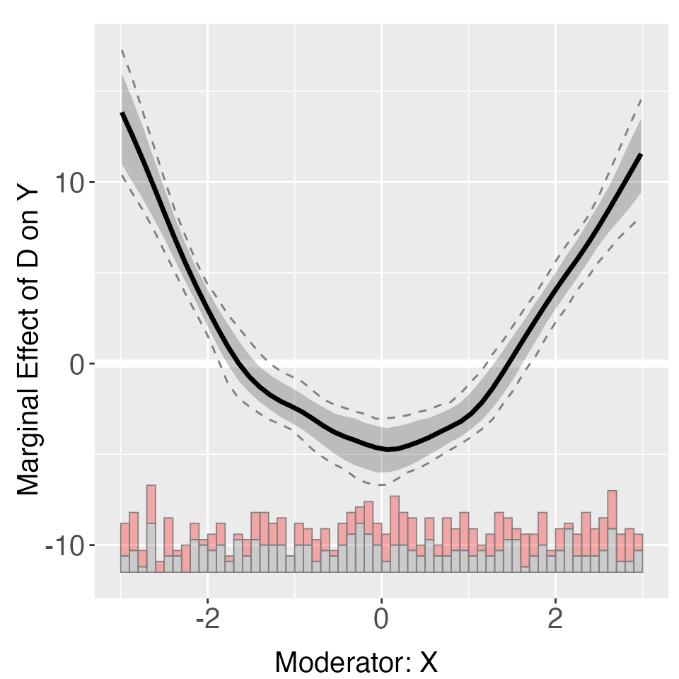

With large datasets, cross-validation or bootstrapping can take a while. One way to check the result quickly is to shut down the bootstrap procedure (using CI = FALSE). interflex will then present the point estimates only. Another way is to supply a reasonable bandwidth manually by using the bw option such that cross-validation will be skipped.

s4.kernel <- interflex(Y = "Y", D = "D", X = "X", Z = "Z1", data = s4, 
                       estimator = "kernel", bw = 0.62, FE = c("unit","year"), cl = "unit", 
                       vartype = 'bootstrap',
                       nboots = 1000, parallel = TRUE, cores = 31,
                       CI = FALSE, ylim = c(-9, 15), theme.bw = TRUE)
plot(s4.kernel)

Multiple (>2) treatment arms

Next, we will show how interflex can be applied when there are more than two condition. First, we plot the raw data:

interflex(estimator = "raw",Y = "Y", D = "D", X = "X", data = s5, ncols = 3)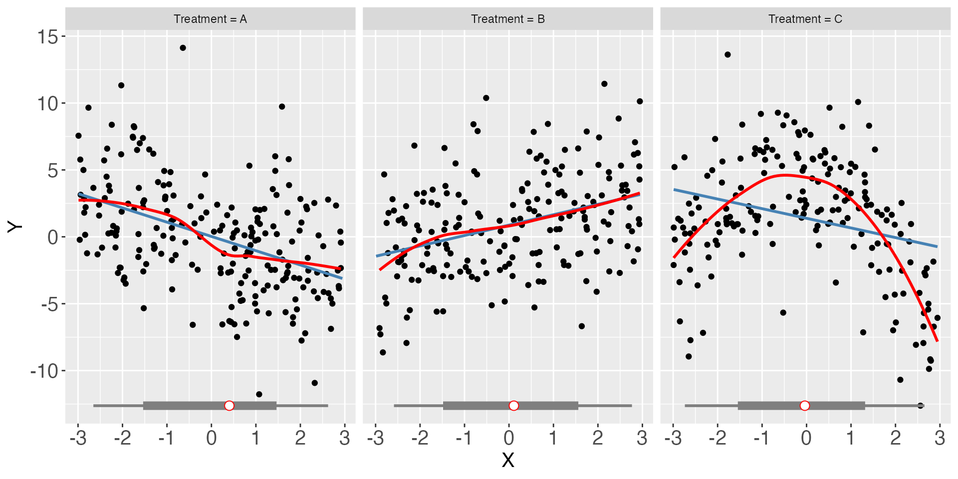

By default, interflex will produce $(n-1)$ marginal effects plots, taking one category as the baseline (if not specified, the base group is selected based on the numeric/character order of the treatment values). Here we also specify vartype = "bootstrap" in order to estimate the confidence intervals.

s5.binning <- interflex(Y = "Y", D = "D", X = "X", Z = c("Z1","Z2"), data = s5, 
                        estimator = "binning", vartype = "bootstrap")
plot(s5.binning)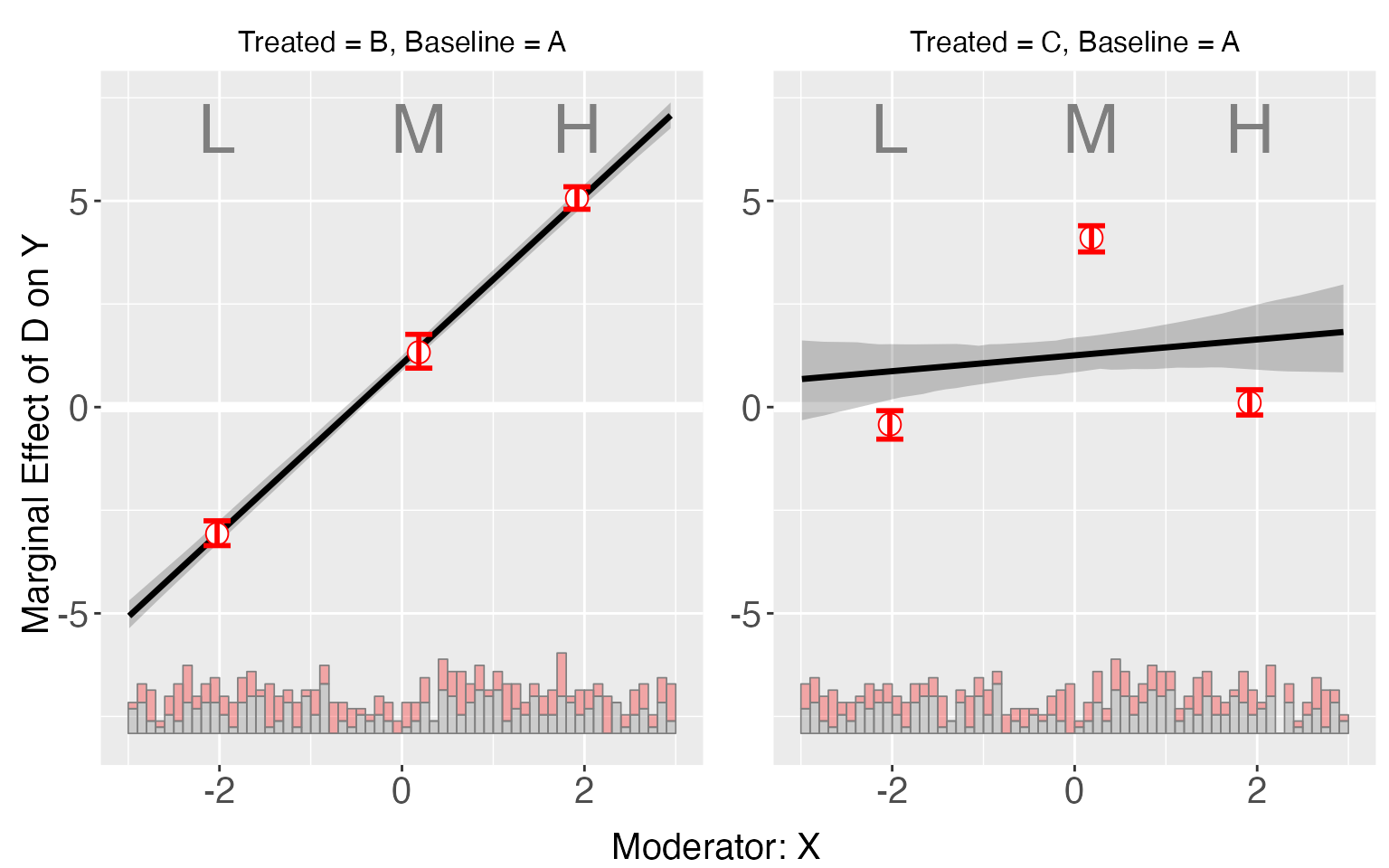

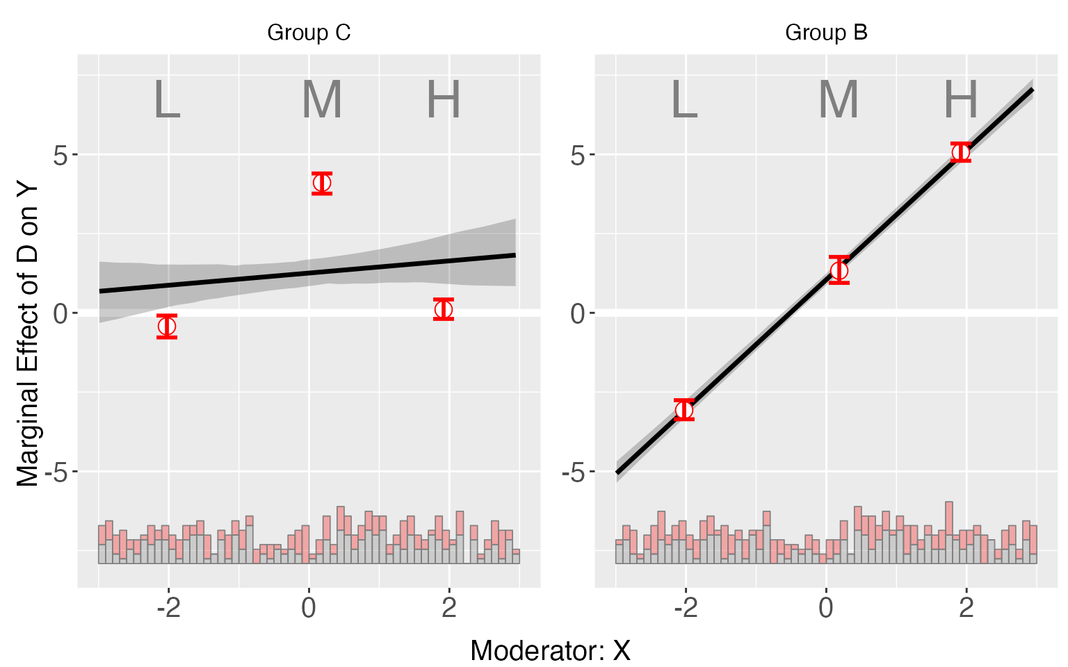
By setting the option order and subtitles (in either interflex or plot), users can also specify the order of plots they prefer and the subtitles they want:

plot(s5.binning, order=c("C", "B"), subtitles = c("Group C","Group B"))

By setting pool = TRUE (in either interflex or plot), we can combine these plots. Users can also specify the colors they like, :

plot(s5.binning, order=c("C", "B"), subtitles = c("Control Group","Group C","Group B"), 
     pool = TRUE, color = c("Salmon","#7FC97F", "#BEAED4"))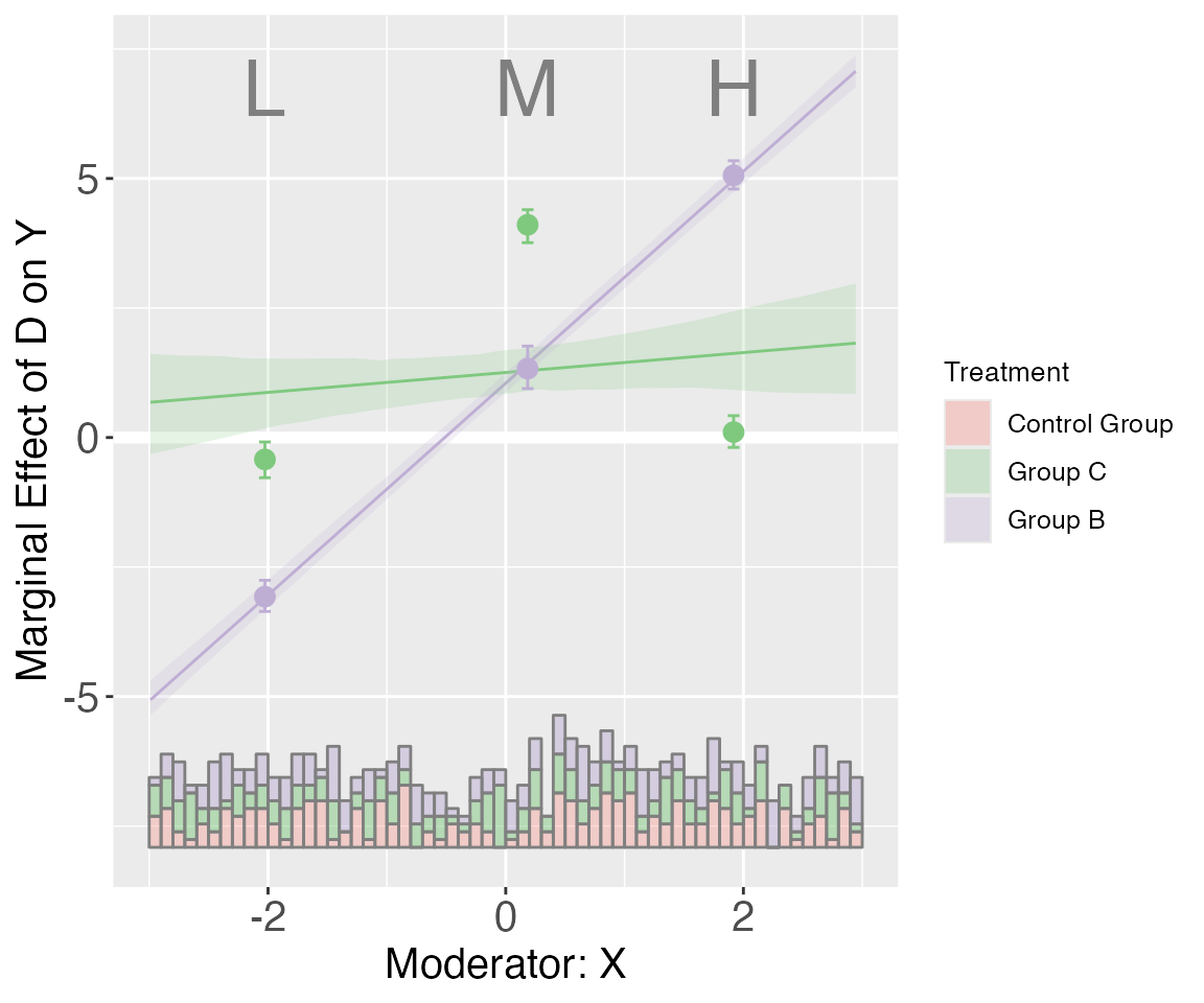

We specify the base group using the option base:

s5.binning2 <- interflex(Y = "Y", D = "D", X = "X",Z = c("Z1", "Z2"), data = s5, 
                         estimator = "binning", base = "B", vartype = "bootstrap")
plot(s5.binning2)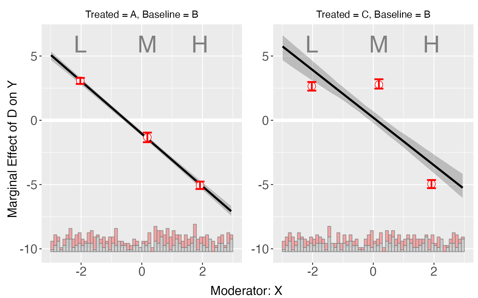

For dataset s5, because of the nonlinear interaction effects, the kernel estimator will produce marginal effects estimates that are much closer to the effects implied by the true DGP.

s5.kernel <- interflex(Y = "Y", D = "D", X = "X",Z = c("Z1", "Z2"), data = s5, 
                       estimator = "kernel", vartype = 'bootstrap',
                       nboots = 1000, parallel = TRUE, cores = 31)
s5.kernel$figure


plot(s5.kernel, pool = TRUE)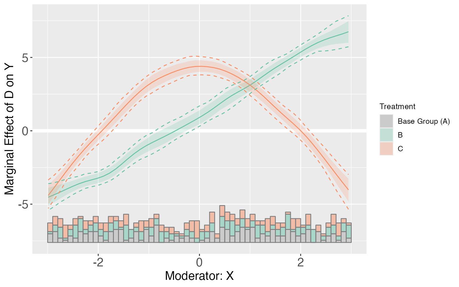

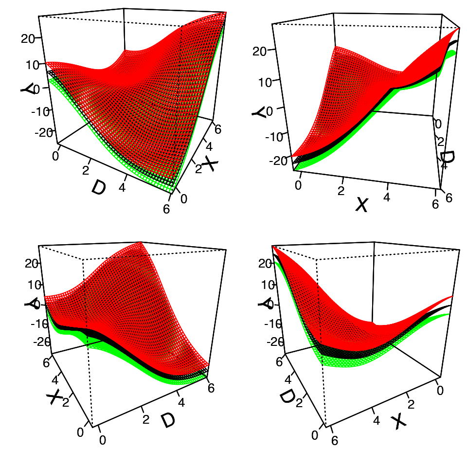
Predicted outcomes

Starting from v.1.1.0, interflex allows users to estimate and visualize predicted outcomes given fixed values of the treatment and moderator based on flexible interaction models. All predictions are made by setting covariates equal to their sample means.

s5.kernel <-interflex(Y = "Y", D = "D", X = "X", Z = c("Z1", "Z2"),
                      data = s5, estimator = "kernel",vartype = 'bootstrap',
                       nboots = 1000, parallel = TRUE, cores = 31)
predict(s5.kernel)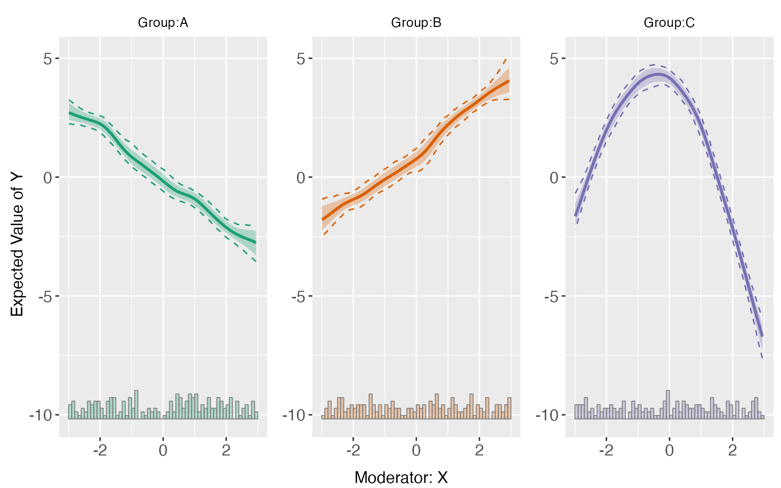

We can also set pool = TRUE to combine them.

predict(s5.kernel,order = c('A','B','C'),subtitle = c("Group A", "Group B", "Group C"), 
        pool = TRUE, legend.title = "Three Different Groups")

We can also use the linear model or the binning model to estimate and visualize predicted outcomes. For the latter, it is expected to see some “zigzags” at the bin boundaries in a plot:

s5.binning <-interflex(Y = "Y", D = "D", X = "X", Z = c("Z1","Z2"), data = s5, 
                       estimator = "binning", vartype = "bootstrap", nbins = 4)
predict(s5.binning)

s5.linear <-interflex(Y = "Y", D = "D", X = "X", Z = c("Z1","Z2"), data = s5, 
                      estimator = "linear", vcov.type = "robust")
predict(s5.linear)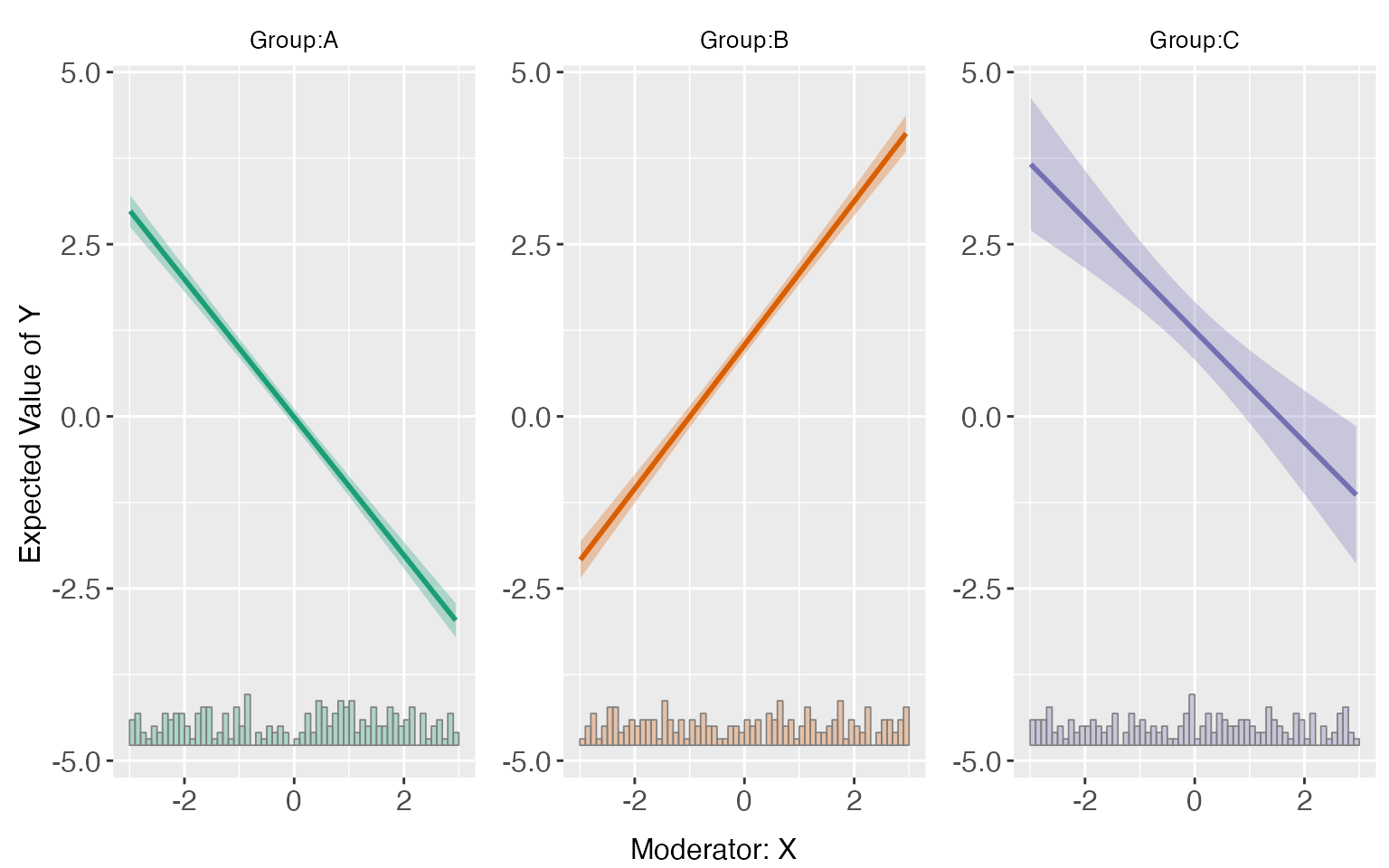

Obviously, the kernel estimator characterizes the data more better than a linear or binning estimator.

Differences in treatment effects

Starting from v.1.1.0, interflex allows users to compare treatment effects at three specific values of the moderator using linear or kernel model. In order to do so, users need to pass three values into diff.values when applying linear or kernel estimator. If not specified, this programme will by default choose the 25,50,75 percentile of the moderator as the diff.values.

s5.kernel <-interflex(Y = "Y", D = "D", X = "X", Z = c("Z1", "Z2"), data = s5, 
                      estimator = "kernel", diff.values = c(-2,0,2),
                      vartype = "bootstrap",
                      nboots = 1000, parallel = TRUE, cores = 31,)
plot(s5.kernel,diff.values = c(-2,0,2))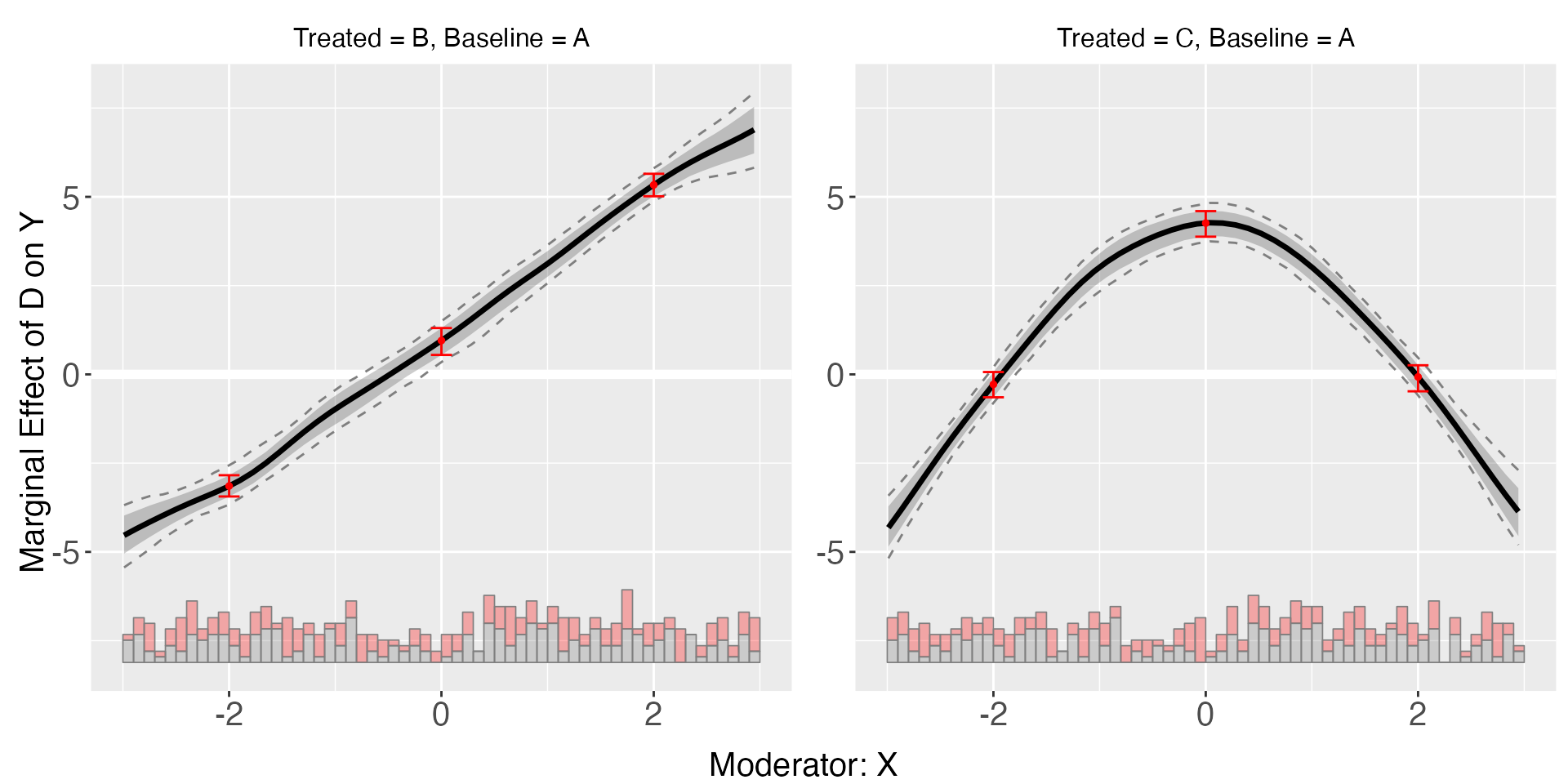

s5.kernel$diff.estimate
#> $B
#>         diff.estimate    sd z-value p-value lower CI(95%) upper CI(95%)
#> 0 vs -2         4.099 0.250  16.380   0.000         3.606         4.561
#> 2 vs 0          4.386 0.258  17.025   0.000         3.900         4.908
#> 2 vs -2         8.485 0.225  37.682   0.000         8.013         8.887
#> 
#> $C
#>         diff.estimate    sd z-value p-value lower CI(95%) upper CI(95%)
#> 0 vs -2         4.550 0.262  17.384   0.000         4.020         5.069
#> 2 vs 0         -4.338 0.260 -16.679   0.000        -4.850        -3.851
#> 2 vs -2         0.212 0.258   0.823   0.410        -0.314         0.678

s5.linear <-interflex(Y = "Y", D = "D", X = "X", Z = c("Z1","Z2"), data = s5, 
                      estimator = "linear", diff.values = c(-2,0,2), 
                      vartype = "bootstrap")
plot(s5.linear,diff.values = c(-2,0,2))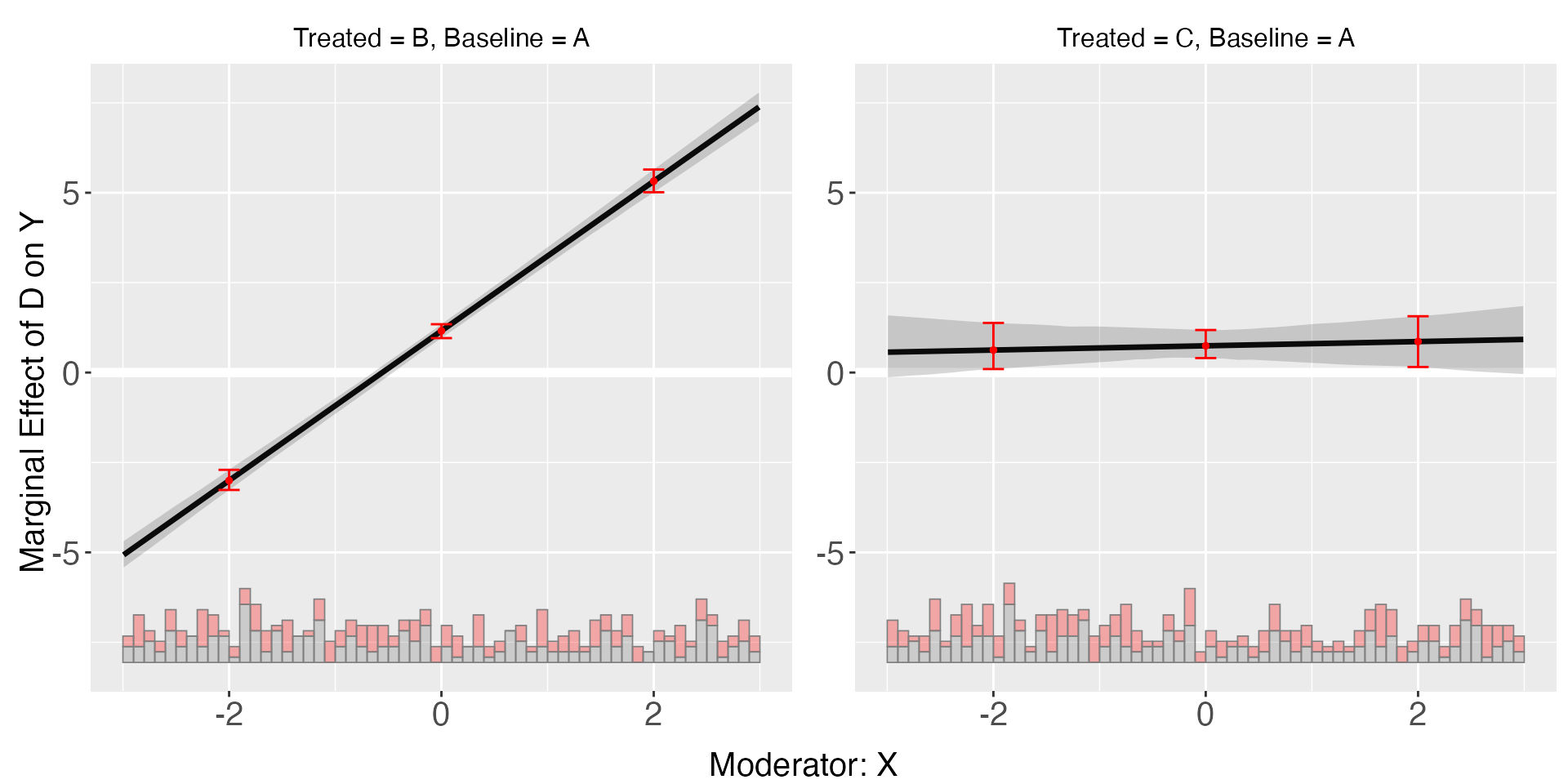

s5.linear$diff.estimate
#> $B
#>         diff.estimate    sd z-value p-value lower CI(95%) upper CI(95%)
#> 0 vs -2         4.090 0.106  38.429   0.000         3.886         4.319
#> 2 vs 0          4.090 0.106  38.429   0.000         3.886         4.319
#> 2 vs -2         8.179 0.213  38.429   0.000         7.772         8.639
#> 
#> $C
#>         diff.estimate    sd z-value p-value lower CI(95%) upper CI(95%)
#> 0 vs -2         0.384 0.293   1.311   0.190        -0.130         0.988
#> 2 vs 0          0.384 0.293   1.311   0.190        -0.130         0.988
#> 2 vs -2         0.769 0.586   1.311   0.190        -0.259         1.975

Starting from v.1.1.1, interflex allows users to compare treatment effects at two or three specific values of the moderator using marginal effects and vcov matrix derived from linear/kernel estimation. Based on GAM model(relies on mgcv package), users can approximate treatment effects and their variance using smooth functions without re-estimating the model, hence saving time. In order to do so, users need to pass the output of interflex into t.test and then specify the values of interest of the moderator. As it is an approximation, the results here are expected to have a little deviance from the output we got by directly specifying diff.values when applying inter.linear or inter.kernel. We also limit the elements passed in diff.values between the minimum and the maximum of the moderator to avoid potential extrapolation bias.

inter.test(s5.kernel,diff.values=c(-2,0,2))
#> $B
#>         diff.estimate    sd z-value p-value lower CI(95%) upper CI(95%)
#> 0 vs -2         4.093 0.250  16.353   0.000         3.603         4.584
#> 2 vs 0          4.389 0.258  17.024   0.000         3.883         4.894
#> 2 vs -2         8.482 0.225  37.614   0.000         8.040         8.924
#> 
#> $C
#>         diff.estimate    sd z-value p-value lower CI(95%) upper CI(95%)
#> 0 vs -2         4.542 0.261  17.396   0.000         4.030         5.054
#> 2 vs 0         -4.332 0.260 -16.682   0.000        -4.841        -3.823
#> 2 vs -2         0.210 0.258   0.814   0.415        -0.295         0.715

inter.test(s5.linear,diff.values=c(-2,0,2))
#> $B
#>         diff.estimate    sd z-value p-value lower CI(95%) upper CI(95%)
#> 0 vs -2         4.090 0.106  38.429   0.000         3.881         4.298
#> 2 vs 0          4.090 0.106  38.429   0.000         3.881         4.298
#> 2 vs -2         8.179 0.213  38.429   0.000         7.762         8.597
#> 
#> $C
#>         diff.estimate    sd z-value p-value lower CI(95%) upper CI(95%)
#> 0 vs -2         0.384 0.293   1.311   0.190        -0.190         0.959
#> 2 vs 0          0.384 0.293   1.311   0.190        -0.190         0.959
#> 2 vs -2         0.769 0.586   1.311   0.190        -0.381         1.918

We can also set percentile = TRUE to use the percentile scale rather than the real scale of the moderator.

inter.test(s5.kernel,diff.values=c(0.25,0.5,0.75),percentile=TRUE)
#> $B
#>            diff.estimate    sd z-value p-value lower CI(95%) upper CI(95%)
#> 50% vs 25%         3.048 0.237  12.836   0.000         2.583         3.514
#> 75% vs 50%         3.270 0.246  13.272   0.000         2.787         3.753
#> 75% vs 25%         6.318 0.235  26.891   0.000         5.858         6.779
#> 
#> $C
#>            diff.estimate    sd z-value p-value lower CI(95%) upper CI(95%)
#> 50% vs 25%         2.736 0.255  10.713   0.000         2.235         3.236
#> 75% vs 50%        -2.561 0.255 -10.026   0.000        -3.062        -2.061
#> 75% vs 25%         0.174 0.264   0.662   0.508        -0.342         0.691