data(hbal)5 Example 2: Black and Owens (2016)
The second example comes from Black and Owens (2016), in which the authors study the effect of promotion prospect to the Supreme Court on the behavior of circuit court judges. Here we focus on whether circuit court judges who are on the shortlist to fill Supreme Court vacancies (“contenders”) ruled in line with the president as the outcome of interest. We load the dataset contenderJudges, which is shipped with hbal.
First, we take a look at the data structure. The outcome variable is presIdeoVote and the treatment variable is treatFinal0, indicating whether there was a Supreme Court vacancy at the time. There are also 7 covariates on judge and court characteristics and a variable judge that indicates the judges’ names.
str(contenderJudges)
#> 'data.frame':    10171 obs. of  10 variables:
#>  $ presIdeoVote: int  0 1 1 1 1 0 0 0 1 0 ...
#>  $ treatFinal0 : int  1 1 1 1 1 1 1 1 1 1 ...
#>  $ judgeJCS    : num  0.28 0.581 0.199 0.406 -0.341 ...
#>  $ presDist    : num  0.0019 0.0552 0.3137 0.2302 0.9772 ...
#>  $ panelDistJCS: num  0.0392 0.562 0.2485 0.4625 0.491 ...
#>  $ circmed     : num  0.0315 0.581 0.0375 0.013 0.047 ...
#>  $ sctmed      : num  0.227 0.122 -0.359 0.122 0.122 ...
#>  $ coarevtc    : int  0 0 0 1 1 1 0 1 0 1 ...
#>  $ casepub     : int  1 1 1 1 1 1 1 1 1 1 ...
#>  $ judge       : Factor w/ 68 levels "Alfred T. Goodwin",..: 34 31 9 4 3 59 67 52 16 34 ...
We can estimate the effect of Supreme Court vacancy on judges’ rulings while controlling for functions of the covariates (to the second order). We see that contender judges are more likely to rule in line with the ideology of the sitting president during a Supreme Court vacancy.
xvars <- c("judgeJCS", "presDist", "panelDistJCS", "circmed", "sctmed", "coarevtc", "casepub")
out <- hbal(Treat = 'treatFinal0', X = xvars, Y = 'presIdeoVote', data = contenderJudges,
            expand.degree = 2, cv = TRUE)
#> Crossvalidation...
summary(out)
#> Call:
#>  hbal(data = contenderJudges, Treat = "treatFinal0", X = xvars,
#>     Y = "presIdeoVote", expand.degree = 2, cv = TRUE)
#>
#>  Treated Controls
#>     4490     5681
#>  Co/Tr Ratio = 1.27
#>
#>  Groups
#>         #Terms Penalty
#> linear       7     0.0
#> squared      5    12.5
#> two-way     21     0.0
#>
#>  Balance Table
#>             Tr.Mean Co.Mean W.Co.Mean Std.Diff.(O) Std.Diff.(W)
#> judge          0.16    0.07      0.16         0.28         0.00
#> presD          0.17    0.45      0.17        -0.91         0.00
#> panel          0.34    0.29      0.34         0.23         0.00
#> circm          0.14    0.00      0.14         0.50         0.00
#> sctme          0.01    0.03      0.01        -0.07         0.00
#> coare          0.28    0.31      0.28        -0.07         0.00
#> casep          0.61    0.84      0.61        -0.53         0.00
#> judge.judge    0.13    0.12      0.15         0.10        -0.19
#> presD.presD    0.06    0.31      0.07        -0.84        -0.04
#> panel.panel    0.18    0.14      0.19         0.18        -0.05
#> circm.circm    0.08    0.08      0.10         0.01        -0.20
#> sctme.sctme    0.04    0.02      0.03         0.40         0.29
#> judge.presD    0.02    0.02      0.02         0.02         0.00
#> judge.panel    0.05    0.03      0.05         0.15         0.00
#> presD.panel    0.04    0.13      0.04        -0.59         0.00
#> judge.circm    0.05    0.05      0.05         0.02         0.00
#> presD.circm    0.01    0.00      0.01         0.08         0.00
#> panel.circm    0.05    0.01      0.05         0.37         0.00
#> judge.sctme   -0.02    0.01     -0.02        -0.54         0.00
#> presD.sctme   -0.01    0.02     -0.01        -0.41         0.00
#> panel.sctme    0.01    0.01      0.01         0.00         0.00
#> circm.sctme    0.01    0.01      0.01        -0.08         0.00
#> judge.coare    0.05    0.02      0.05         0.13         0.00
#> presD.coare    0.05    0.14      0.05        -0.39         0.00
#> panel.coare    0.10    0.09      0.10         0.04         0.00
#> circm.coare    0.03    0.00      0.03         0.21         0.00
#> sctme.coare    0.01    0.01      0.01        -0.02         0.00
#> judge.casep    0.10    0.04      0.10         0.23         0.00
#> presD.casep    0.12    0.37      0.12        -0.83         0.00
#> panel.casep    0.21    0.24      0.21        -0.09         0.00
#> circm.casep    0.05   -0.02      0.05         0.30         0.00
#> sctme.casep    0.00    0.01      0.00        -0.09         0.00
#> coare.casep    0.22    0.30      0.22        -0.16         0.00
att(out)
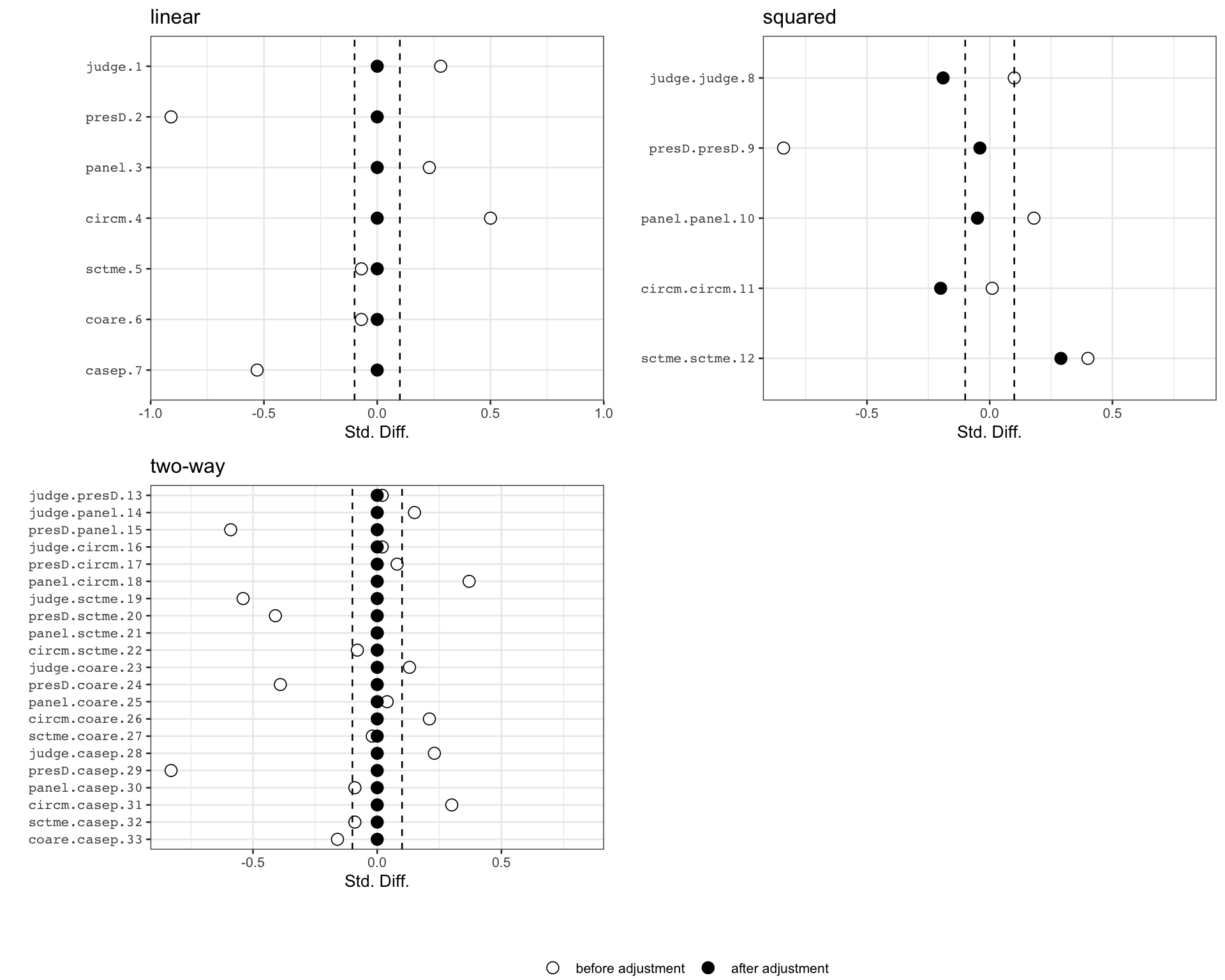
We can further check covariate balance before and after balancing by checking the balance plots. Here we see that the linear terms are exactly balanced between the treatment and the control groups. Imbalance among higher-order terms and interactions are also significantly reduced.
plot(out)