4 Example 1: Lalonde Data
To show the use of habl in practice, here we use habl on a dataset that contains the subset of the LaLonde (1986) dataset from Dehejia and Wahba (1999) and the Panel Study of Income Dynamics (PSID-1), which is also shipped with hbal.
First, we adjust for the linear terms only:
xvars <- c("age","black","educ","hisp","married","re74","re75","nodegr","u74","u75") # covariates
# hbal w/ level terms only
hbal.out <- hbal(Treat = 'nsw', X = xvars,  Y = 're78', data = lalonde)
summary(hbal.out)
#> Call:
#>  hbal(data = lalonde, Treat = "nsw", X = xvars, Y = "re78")
#>
#>  Treated Controls
#>      185     2490
#>  Co/Tr Ratio = 13.46
#>
#>  Groups
#>        #Terms Penalty
#> linear     10       0
#>
#>  Balance Table
#>       Tr.Mean  Co.Mean W.Co.Mean Std.Diff.(O) Std.Diff.(W)
#> age     25.82    34.85     25.82        -0.86            0
#> black    0.84     0.25      0.84         1.30            0
#> educ    10.35    12.12     10.35        -0.58            0
#> hisp     0.06     0.03      0.06         0.15            0
#> marri    0.19     0.87      0.19        -1.76            0
#> re74  2095.57 19428.75   2100.16        -1.26            0
#> re75  1532.06 19063.34   1536.82        -1.26            0
#> nodeg    0.71     0.31      0.71         0.85            0
#> u74      0.71     0.09      0.71         1.85            0
#> u75      0.60     0.10      0.60         1.46            0
att(hbal.out)
Next, we add higher-order terms. The confidence intervals of both estimates cover the experimental benchmark (~$1800). As a result of cross-validation, no penalty is imposed on the linear and squared terms. Note that exclude=list(c("educ", "nodegr")) removes the nonsensical interaction between educ and nodegr.
hbal.full.out <- hbal(Treat = 'nsw', X = xvars, Y = 're78', data = lalonde,
                      expand.degree = 2, cv = TRUE, exclude=list(c("educ", "nodegr")))
#> Crossvalidation...
#> Matrix inversion resulted in large error.
#> Matrix inversion resulted in large error.
#> Matrix inversion resulted in large error.
#> Matrix inversion resulted in large error.
#> Matrix inversion resulted in large error.
#> Matrix inversion resulted in large error.
#> Matrix inversion resulted in large error.
#> Matrix inversion resulted in large error.
#> Matrix inversion resulted in large error.
summary(hbal.full.out)
#> Call:
#>  hbal(data = lalonde, Treat = "nsw", X = xvars, Y = "re78", expand.degree = 2,
#>     cv = TRUE, exclude = list(c("educ", "nodegr")))
#>
#>  Treated Controls
#>      185     2490
#>  Co/Tr Ratio = 13.46
#>
#>  Groups
#>         #Terms Penalty
#> linear      10     0.0
#> squared      4     0.6
#> two-way     42   100.0
#>
#>  Balance Table
#>                 Tr.Mean      Co.Mean   W.Co.Mean Std.Diff.(O) Std.Diff.(W)
#> age               25.82        34.85       25.82        -0.86         0.00
#> black              0.84         0.25        0.84         1.30         0.00
#> educ              10.35        12.12       10.35        -0.58         0.00
#> hisp               0.06         0.03        0.06         0.15         0.00
#> marri              0.19         0.87        0.19        -1.76         0.00
#> re74            2095.57     19428.75     2099.90        -1.26         0.00
#> re75            1532.06     19063.34     1536.55        -1.26         0.00
#> nodeg              0.71         0.31        0.71         0.85         0.00
#> u74                0.71         0.09        0.71         1.85         0.00
#> u75                0.60         0.10        0.60         1.46         0.00
#> age.age          717.39      1323.53      731.32        -0.79        -0.02
#> educ.educ        111.06       156.32      112.75        -0.64        -0.02
#> re74.re74   28141434.44 557148332.57 25601663.05        -0.62         0.00
#> re75.re75   12654752.23 548213776.79 12199535.33        -0.60         0.00
#> age.black         21.91         8.56       21.37         0.84         0.03
#> age.educ         266.98       414.70      260.62        -0.95         0.04
#> black.educ         8.70         2.60        8.37         1.23         0.07
#> age.hisp           1.36         1.16        1.59         0.03        -0.03
#> educ.hisp          0.58         0.35        0.75         0.11        -0.08
#> age.marri          5.56        30.90        6.50        -1.53        -0.06
#> black.marri        0.16         0.20        0.12        -0.10         0.09
#> educ.marri         1.96        10.47        1.95        -1.57         0.00
#> hisp.marri         0.02         0.03        0.01        -0.08         0.02
#> age.re74       54074.04    704912.21    53307.79        -1.07         0.00
#> black.re74      1817.20      3646.09     1716.49        -0.24         0.01
#> educ.re74      22898.73    248073.37    22824.07        -1.08         0.00
#> hisp.re74        151.40       589.15      123.66        -0.12         0.01
#> marri.re74       760.63     17578.61      842.05        -1.15        -0.01
#> age.re75       41167.28    688282.61    37674.97        -1.07         0.01
#> black.re75      1257.04      3502.23     1318.58        -0.30        -0.01
#> educ.re75      15880.57    244584.33    16252.51        -1.09         0.00
#> hisp.re75        153.73       511.72       43.71        -0.10         0.03
#> marri.re75       654.34     17200.24      492.48        -1.13         0.01
#> re74.re75   13118590.79 523653961.37 11663711.60        -0.62         0.00
#> age.nodeg         17.97        11.83       18.48         0.33        -0.03
#> black.nodeg        0.61         0.13        0.67         1.28        -0.15
#> educ.nodeg         6.71         2.62        6.60         0.95         0.03
#> hisp.nodeg         0.05         0.01        0.02         0.27         0.25
#> marri.nodeg        0.14         0.26        0.11        -0.28         0.07
#> re74.nodeg      1094.15      4511.11     1189.29        -0.40        -0.01
#> re75.nodeg      1134.96      4272.56     1008.29        -0.37         0.02
#> age.u74           18.78         3.50       18.63         1.22         0.01
#> black.u74          0.60         0.01        0.59         2.57         0.05
#> educ.u74           7.26         1.01        7.34         1.60        -0.02
#> hisp.u74           0.03         0.00        0.05         0.39        -0.20
#> marri.u74          0.11         0.07        0.10         0.15         0.03
#> re75.u74         307.44       372.31      299.38        -0.02         0.00
#> nodeg.u74          0.52         0.03        0.51         2.01         0.05
#> age.u75           15.98         3.99       16.47         0.93        -0.04
#> black.u75          0.52         0.02        0.52         2.15        -0.02
#> educ.u75           6.15         1.15        6.28         1.26        -0.03
#> hisp.u75           0.03         0.01        0.02         0.27         0.14
#> marri.u75          0.09         0.09        0.12         0.00        -0.12
#> re74.u75          43.85       483.27      384.01        -0.13        -0.10
#> nodeg.u75          0.43         0.04        0.44         1.58        -0.02
#> u74.u75            0.59         0.07        0.53         1.74         0.20
att(hbal.full.out)
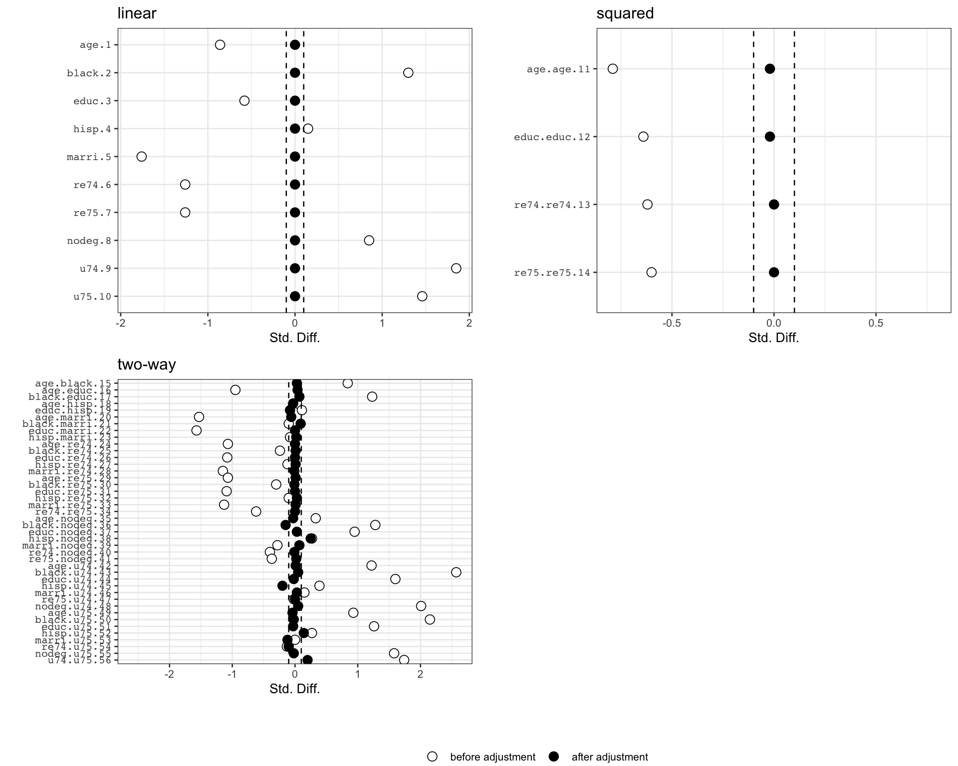
We can check the penalties applied to each group and the cavariate balance before and after balancing.
hbal.full.out$group.penalty
#>      linear     squared     two-way
#>   0.0000000   0.6168256 100.0000000
plot(hbal.full.out)