library(hbal)
set.seed(1984)
N <- 1500
X1 <- rnorm(N)
X2 <- rnorm(N)
X3 <- rbinom(N, size = 1, prob = .5)
D_star <- 0.5 * X1 + 0.3 * X2 + 0.2 * X1 * X2 - 0.5 * X1 * X3 - 1
D <- ifelse(D_star > rnorm(N), 1, 0) # Treatment indicator
y <- 0.5 * D + X1 + X2 + X2 * X3 + rnorm(N) # Outcome
dat <- data.frame(D = D, X1 = X1, X2 = X2, X3 = X3, Y = y)
head(dat)1 Basic Usage
We simulate a toy cross-sectional dataset with a binary treatment to illustrate the basic usage of hbal. Note that treatment assignment depends on all three covariates.
hbal is an extension of entropy balancing, or ebal proposed by Hainmueller (2012). By default, hbal replicates ebal by performing exact balancing on all covariates and no serial expansion, i.e., expand.degree = 1 (default). We can demonstrate this equivalence by showing the hbal weights are exactly the same to the ebal weights from the ebal package in this case.
library(ebal)
ebal.out <- ebalance(Treat = dat$D, X = dat[,c('X1', 'X2', 'X3')]) # ebal
hbal.out <- hbal(Treat = 'D', X = c('X1', 'X2', 'X3'),  Y = 'Y',  data = dat) # hbal

# plot weights
W <- data.frame(x = ebal.out$w, y = hbal.out$weights.co)
ggplot(aes(x = x, y = y), data = W) + geom_point() + theme_bw() +
  labs(x = "ebal weights", y="hbal weights", title = "ebal weights vs. hbal weights")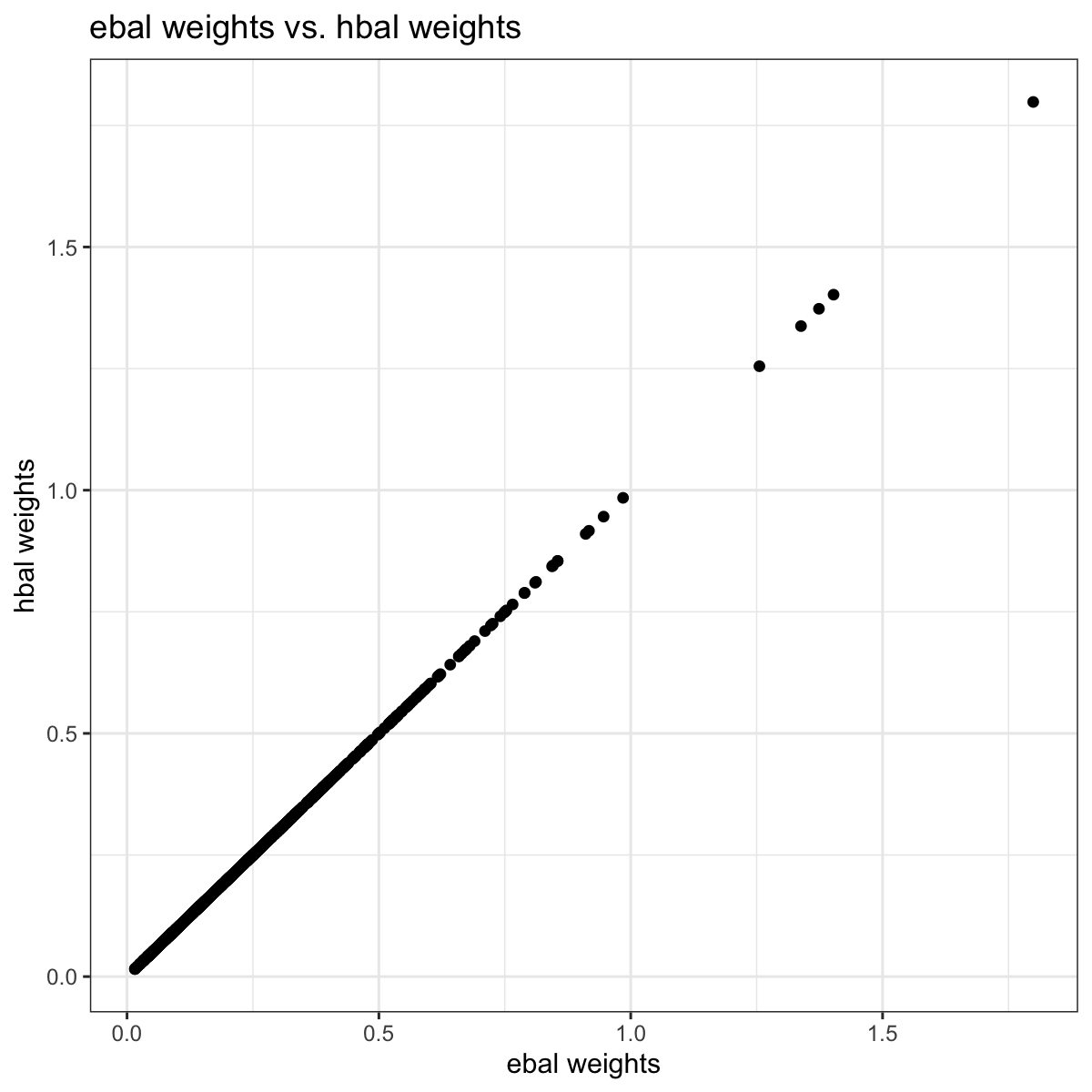
hbal() returns a list of 15 objects:
names(hbal.out)
#>  [1] "converged"     "weights"       "weights.co"    "coefs"
#>  [5] "Treatment"     "mat"           "grouping"      "group.penalty"
#>  [9] "term.penalty"  "bal.tab"       "base.weights"  "Treat"
#> [13] "Outcome" "Y" "call"- converged: Binary indicator of whether the algorithm has converged.
- weights: Resulting weights, including the base weights for the treated and solution weights for the controls (see below).
- weights.co: Solution weights for the controls. Can be plugged into any downstream estimator.
-
coefs: Values of Lagrangian multipliers. They are used to calculate the solution
weights. - Treatment: The treatment status vector.
- mat: Data matrix, including the outcome variable (the first column), the treatment variable (the second column), and expanded covariates (the remaining columns).
- grouping: A vector of the number of variables in each covariate group. The length of the vector equals the number of groups.
- group.penalty: Penalties for different groups of covariates. This is the regularization parameter \(\alpha\) in Xu and Yang (2022).
- term.penalty: Penalties for individual covariates. The length of the vector equals the number of balancing terms, including expanded ones.
- bal.tal: A balance table.
-
base.weights: A vector of base weights, originally from variable
wsupplied by users. The length of the vector equals the number of rows entering the balancing scheme. - Treat: A character string that stores the treatment variable name.
-
Outcome: The outcome vector, if
Yis supplied. -
Y: A character string that stores the outcome variable name, if
Yis supplied.. - call: A string of the function call.
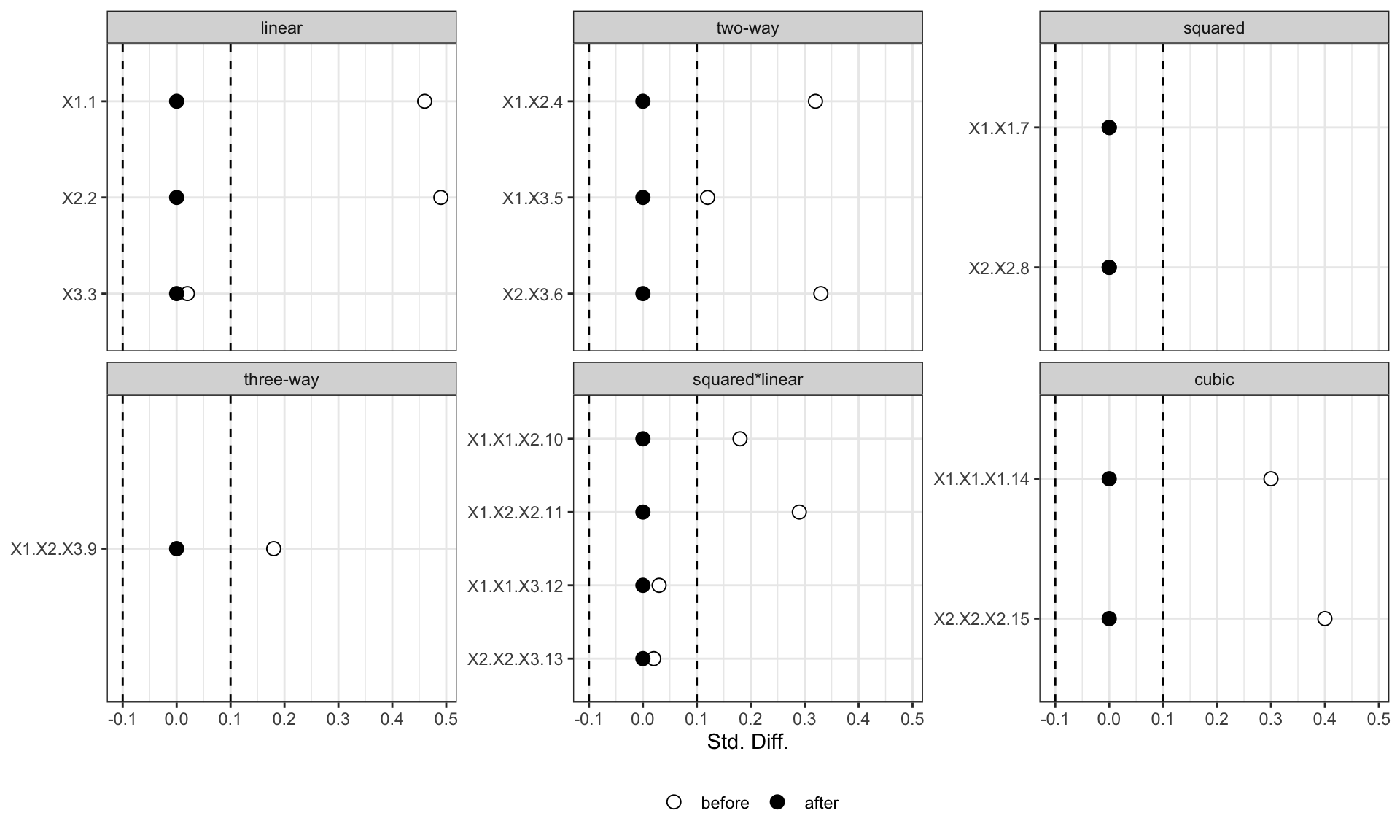
The summary() function provides additional information on the balancing scheme, including the numbers of treated and control units, groups and corresponding penalties, and a balance table, in which Std.Diff.(O) and Std.Diff.(W) represent standardized difference before and after balancing, respectively. For example, in this case, only the linear terms are being balanced on.
summary(hbal.out)
#> Call:
#>  hbal(data = dat, Treat = "D", X = c("X1", "X2", "X3"), Y = "Y")
#>
#>  Treated Controls
#>      256     1244
#>  Co/Tr Ratio = 4.86
#>
#>  Groups
#>        #Terms Penalty
#> linear      3       0
#>
#>  Balance Table
#>    Tr.Mean Co.Mean W.Co.Mean Std.Diff.(O) Std.Diff.(W)
#> X1    0.35   -0.11      0.35         0.46            0
#> X2    0.42   -0.07      0.42         0.49            0
#> X3    0.52    0.51      0.52         0.02            0
In addition to balancing on just the linear/level terms of the covariates, hbal() allows balancing on a serial expansion of the covariates. This is achieved by setting the expand.degree argument. Currently, hbal() supports both second order serial expansion (two-way interactions and square terms; expand.degree = 2) and third order serial expansion (two-way interactions, square terms, linear*square interactions, and cubic terms; expand.degree = 3). For example, we can do exact balancing on third order serial expansion of the covariates:
out <- hbal(Y = 'Y', Treat = 'D', X = c('X1', 'X2', 'X3'),
            data = dat, expand.degree = 3)
summary(out)
#> Call:
#>  hbal(data = dat, Treat = "D", X = c("X1", "X2", "X3"), Y = "Y",
#>     expand.degree = 3)
#>
#>  Treated Controls
#>      256     1244
#>  Co/Tr Ratio = 4.86
#>
#>  Groups
#>                #Terms Penalty
#> linear              3       0
#> two-way             3       0
#> squared             2       0
#> three-way           1       0
#> squared*linear      4       0
#> cubic               2       0
#>
#>  Balance Table
#>          Tr.Mean Co.Mean W.Co.Mean Std.Diff.(O) Std.Diff.(W)
#> X1          0.35   -0.11      0.35         0.46            0
#> X2          0.42   -0.07      0.42         0.49            0
#> X3          0.52    0.51      0.52         0.02            0
#> X1.X2       0.24   -0.10      0.24         0.32            0
#> X1.X3       0.07   -0.02      0.07         0.12            0
#> X2.X3       0.21   -0.01      0.21         0.33            0
#> X1.X1       1.01    1.01      1.01         0.00            0
#> X2.X2       0.99    0.99      0.99         0.00            0
#> X1.X2.X3    0.13    0.00      0.13         0.18            0
#> X1.X1.X2    0.32   -0.01      0.32         0.18            0
#> X1.X2.X2    0.32   -0.17      0.32         0.29            0
#> X1.X1.X3    0.55    0.52      0.55         0.03            0
#> X2.X2.X3    0.50    0.47      0.50         0.02            0
#> X1.X1.X1    0.93   -0.25      0.93         0.30            0
#> X2.X2.X2    1.16   -0.23      1.16         0.40            0
1.1 Custom balance plots with balanceData()
plot() draws the balance figure for you. When you want a different figure, balanceData() returns the numbers it draws.
bd <- balanceData(out)
head(bd)
Every term of the expanded covariate matrix gets two rows, one before weighting and one after. std.diff is the standardized difference in means, covar.group is the expansion group the term belongs to, and tr.mean, co.mean and w.co.mean are the treated mean and the control mean before and after weighting. From this data frame you can restyle the figure, keep only the groups you care about, or show a handful of covariates instead of all of them.
bd$term <- factor(bd$term, levels = rev(unique(bd$term)))

ggplot(bd, aes(x = std.diff, y = term, fill = adjustment)) +
  geom_vline(xintercept = c(-0.1, 0.1), linetype = 2) +
  geom_point(size = 3, shape = 21, colour = "black") +
  scale_fill_manual(values = c(before = "white", after = "black")) +
  facet_wrap(~ covar.group, scales = "free_y") +
  labs(x = "Std. Diff.", y = NULL) +
  theme_bw() +
  theme(legend.title = element_blank(), legend.position = "bottom")