att(out)att(out, method = "lm_robust")att(out, method = "lm_lin", se_type = "stata")att(out, dr = FALSE)We can use att() on an hbal object to get an ATT estimate.
method = "abw")Since version 1.3.0, the default estimator is an augmented balancing weights estimator (method = "abw"; Ben-Michael et al. (2021), Bruns-Smith et al. (2023)). It combines the hbal weights with an outcome model in three steps:
Fit a regression of the outcome on the columns of mat, using the control units only and weighted by their hbal weights. The regression is a ridge regression on standardized columns with an unpenalized intercept. Its penalty is chosen once from the full control sample by generalized cross-validation (Golub et al. 1979) over a fixed grid, with a cap on the effective degrees of freedom so that the fit can never interpolate the controls. No random numbers are involved.
Predict the untreated outcome of each treated unit from that regression. Then correct the prediction with the hbal-weighted average of the control residuals. The residual term corrects the regression where it is wrong; the regression corrects the weights where the balance is only approximate.
Take the weighted mean of the treated outcomes and subtract the corrected prediction.
The resulting estimator is doubly robust. It is also Neyman-orthogonal: a small error in either the outcome regression or the weights has no first-order effect on the estimate. The control residuals in step 2 are cross-fitted: the controls are split into folds, and each control’s residual comes from a regression fitted without its own fold. Standard errors come from the influence function of the estimator, treating the weights and the outcome regression as fixed; the p-value and the 95 percent confidence interval use a t distribution with n − 1 degrees of freedom.
If the entropy-balancing algorithm did not converge (out$converged is 0), att()’s default method warns that the estimate and its standard error may be unreliable. The warning names the usual remedies: refit hbal() with cv = TRUE, a lower expand.degree, or the ds, X.keep, or exclude options.
| Argument | Default | What it does |
|---|---|---|
method |
"abw" |
Which estimator to use: "abw" (default, above), "lm_robust", "lm_lin", or "elnet" (below). |
dr |
TRUE |
Whether to include the outcome model. FALSE drops it for every method, which then returns the weighted difference in means. "abw" and "lm_robust" compute it directly; "lm_lin" and "elnet" are defined only with an outcome model, so att() estimates them as "lm_robust". |
nfolds |
5 |
Number of cross-fitting folds for method = "abw". att() uses fewer, and says so in a message, when the control group is small relative to the number of columns in mat. Ignored by the other methods. |
seed |
NULL |
Fixes the cross-fitting fold assignment for method = "abw". The assignment is a deterministic function of seed; att() never calls set.seed(), so results are identical across repeated calls with or without a seed. Ignored by the other methods. |
displayAll |
FALSE |
FALSE returns the one-row summary table. TRUE returns the full result instead: a list for "abw" (see above), the fitted model object for "lm_robust"/"lm_lin". |
... |
— | Extra arguments, forwarded to lm_robust()/lm_lin() (e.g. se_type, clusters). method = "abw" does not accept any and stops with an error naming them. |
The three estimators available before version 1.3.0 remain available through the method argument and give exactly the numbers they gave before:
method = "lm_robust": weighted linear regression with robust standard errors, using lm_robust() from the estimatr package. This was the default before version 1.3.0. Set it explicitly to reproduce results from earlier versions.
method = "lm_lin": weighted linear regression with a full set of interactions between the treatment indicator and the demeaned covariates, or Lin’s method (Lin 2013), using lm_lin() from estimatr.
method = "elnet": approximate residual balancing (Athey et al. 2018), which fits an elastic-net outcome model with glmnet.
Additional arguments accepted by lm_robust() or lm_lin(), such as se_type and clusters, can be passed to att() with those two methods only. The default method does not accept them and stops with an error that points to method = "lm_robust" or "lm_lin". Setting dr = FALSE drops the outcome model, and every method then returns the same estimate: the difference in weighted means. The default method and method = "lm_robust" compute it directly and differ only in how the standard error is computed. method = "lm_lin" and method = "elnet" are defined only with an outcome model, so with dr = FALSE they are estimated as "lm_robust" and return its estimate, standard error and degrees of freedom. Before version 1.3.0 those two methods accepted dr = FALSE and silently ignored it; version 1.3.0 fixes that. Note that att(out, dr = FALSE) now uses the default method, so add method = "lm_robust" to reproduce the standard errors from earlier versions.
att(out)att(out, method = "lm_robust")att(out, method = "lm_lin", se_type = "stata")att(out, dr = FALSE)Under dr = FALSE the three legacy methods return one and the same row, because "lm_lin" and "elnet" are estimated as "lm_robust".
att(out, method = "lm_robust", dr = FALSE)att(out, method = "lm_lin", dr = FALSE)att(out, method = "elnet", dr = FALSE)By default, att() only displays the treatment effect (displayAll = FALSE). With displayAll = TRUE, the default method returns a list with the estimate, its standard error, the per-unit influence values, the fold assignment, the coefficients of the outcome regression, and the weights. For method = "lm_robust" or "lm_lin", displayAll = TRUE returns the fitted estimatr object instead.
res <- att(out, displayAll = TRUE)
str(res, max.level = 1)
#> List of 10
#>  $ estimate : num 0.472
#>  $ se       : num 0.0738
#>  $ df       : num 1499
#>  $ method   : chr "abw"
#>  $ dr       : logi TRUE
#>  $ influence: num [1:1500] 0.9802 0.6757 1.0872 0.0495 -1.1783 ...
#>  $ fold     : int [1:1500] 1 NA 2 3 4 5 1 2 3 NA ...
#>  $ nfolds   : int 5
#>  $ nuisance :List of 3
#>  $ weights  :List of 2
round(res$nuisance$coef_full, 3)
#> (Intercept)        X1.1        X2.2        X3.3     X1.X2.4     X1.X3.5
#>       0.094       0.995       1.006      -0.094       0.103       0.044
#>     X2.X3.6     X1.X1.7     X2.X2.8  X1.X2.X3.9 X1.X1.X2.10 X1.X2.X2.11
#>       1.056      -0.048       0.040      -0.080       0.000      -0.008
#> X1.X1.X3.12 X2.X2.X3.13 X1.X1.X1.14 X2.X2.X2.15
#> 0.037 -0.003 -0.012 -0.025method = "abw" (the default) for inference: its 95 percent coverage is 0.945 to 0.956 across the sample sizes and the two main scenarios in the simulations below.
method = "lm_robust", with no other arguments changed, to reproduce a result computed with hbal before version 1.3.0 exactly — point estimate and standard error both.
method = "lm_robust", se_type = "HC3" for a new small-sample analysis (N of 500 or fewer) that uses the pre-1.3.0 point estimate but wants a better-calibrated standard error than its pre-1.3.0 default provides; see below for why.
nfolds = 1 only when a smaller root-mean-squared error matters more than a reliable standard error, and the sample is small; see below for the trade-off.
method = "elnet" for a high-dimensional expansion (many covariates, or a high expand.degree); this method was not part of the simulations below.
Simulations accompanying the 1.3.0 release compare method = "abw" (the default) against method = "lm_robust" (the pre-1.3.0 default) across three data-generating processes and three sample sizes (N = 200, 500, 1000), 1,000 replications per cell.
Small samples. At N = 200, the default’s root-mean-squared error (RMSE) is higher than lm_robust’s: 0.216 vs 0.189 (14 percent higher) when the outcome model is right and the weights are only approximately balanced, and 0.227 vs 0.169 (34 percent higher) when both the weights and the outcome model are mildly wrong. The gap narrows as N grows: by N = 1000 it is 0.087 vs 0.086 and 0.082 vs 0.080, both under 3 percent. In exchange, the default’s standard errors are calibrated when the outcome model is right: an SE ratio (mean estimated standard error divided by the actual spread of the estimates across replications) of 0.99 to 1.00 and 95 percent coverage of about 0.95 (0.948 to 0.956), at every N. lm_robust’s standard error there runs 5 to 7 percent short at every N, not only at N = 200 (SE ratio 0.93 to 0.95; coverage 0.93 to 0.945).
nfolds = 1 (no cross-fitting). Setting nfolds = 1 turns off cross-fitting, and the residual-correction term in step 2 becomes identically zero: what att() returns is then exactly the hbal-weighted ridge regression’s prediction of the treated units’ counterfactual outcome, with no correction step. At N = 200 this closes most of the small-sample RMSE gap to lm_robust: RMSE falls from 0.216 to 0.200 when the outcome model is right (59 percent of the gap to lm_robust’s 0.189), and from 0.227 to 0.190 when both nuisances are mildly wrong (64 percent of the gap to lm_robust’s 0.169). The cost is the standard error: at N = 200 the SE ratio drops to 0.93 (from the default’s 0.995) when the outcome model is right, and to 0.89 (from 0.924) when both nuisances are wrong, and 95 percent coverage falls to 0.935 and 0.921 respectively (both below the default’s 0.956). Under the mildly misspecified scenario, nfolds = 1’s bias is also larger than the default’s at every N (0.031 to 0.033 vs 0.011 to 0.025), because cross-fitting is what supplies the finite-sample correction that shrinks it. Ten folds do no better than the default five — RMSE stays within 2.3 percent of the five-fold value at every N in these two scenarios — so five remains the default.
Standard errors for method = "lm_robust". Its default standard error (se_type = "stata", equivalent to HC1 with no clusters) runs short when the outcome model is right: an SE ratio of 0.93 to 0.95, 4.7 to 7.2 percent short of calibrated, at every N tested. Setting se_type = "HC3" closes most of this gap at N of 500 or fewer (SE ratio 0.997 to 1.042, coverage 0.949 to 0.956) but still leaves the standard error about 5 percent short at N = 1000 (SE ratio 0.951, coverage 0.938). This remaining shortfall is not a small-sample leverage effect: the leverage correction itself shrinks with N as it should (HC3 adds only 2.5 percent to the standard error at N = 1000, against 9.7 percent at N = 200), while the part of the shortfall that survives at N = 1000 does not shrink that way. A plausible source, not tested here, is that the standard-error formula treats the estimated hbal weights as fixed.
The table below compares the default and lm_robust directly, at N = 200 and N = 1000, in the two scenarios above (true ATT: 2 in the first, 1.593 in the second; N = 500, not shown, gives the same coverage ordering: 0.954 vs 0.941 in the first scenario, 0.947 vs 0.935 in the second).
| Scenario | N | Method | Bias | SE ratio | 95% coverage |
|---|---|---|---|---|---|
| Weights approximate, outcome model right | 200 | abw (default) | -0.018 | 0.995 | 0.956 |
| Weights approximate, outcome model right | 200 | lm_robust | 0.001 | 0.950 | 0.945 |
| Weights approximate, outcome model right | 1000 | abw (default) | -0.001 | 0.992 | 0.948 |
| Weights approximate, outcome model right | 1000 | lm_robust | 0.000 | 0.928 | 0.929 |
| Both nuisances mildly wrong | 200 | abw (default) | 0.011 | 0.924 | 0.956 |
| Both nuisances mildly wrong | 200 | lm_robust | 0.023 | 0.984 | 0.941 |
| Both nuisances mildly wrong | 1000 | abw (default) | 0.025 | 1.012 | 0.945 |
| Both nuisances mildly wrong | 1000 | lm_robust | 0.030 | 0.989 | 0.927 |
Both methods are close to unbiased when only the weights are approximately balanced; when the outcome model is also wrong, the default’s bias is about half of lm_robust’s at N = 200 (0.011 vs 0.023) but its standard error is the less calibrated of the two there (SE ratio 0.924 vs 0.984). By N = 1000 the default’s standard error is calibrated in both scenarios (0.99 to 1.01) while lm_robust’s remains 1 to 7 percent short and its coverage 0.927 to 0.929, short of the nominal 95 percent.
A third scenario (not shown above) makes the confounding a nonlinear function of the observed covariates, severe enough that no polynomial expansion of mat can represent it. There, neither estimator is consistent, but the default’s bias is smaller at every N (1.74 vs 2.32 at N = 200) while its spread is larger (SD 8.89 vs 2.46 at N = 200, narrowing to 2.28 vs 1.01 by N = 1000).
Furthermore, hbal() allows variable penalties on the balancing conditions for different groups of covariates. Penalties are automatically determined using cross-validation. This minimizes the variance of the weights, increases the feasibility of the balancing problem, and is the approach advocated in Xu and Yang (2022). We can do so by setting cv = TRUE. Note that, by default, hbal() only penalizes higher-order terms and seeks to achieve exact balance on linear terms. Cross-validation draws random numbers, so a cv = TRUE fit is not reproducible unless you pass a seed. seed = 94035 is the value hbal() set internally up to version 1.2.15, so it reproduces the cross-validated results of those versions.
out <- hbal(Treat = 'D', X = c('X1', 'X2', 'X3'),  Y = 'Y',
            data = dat, expand.degree = 3, cv = TRUE, seed = 94035)
#> Crossvalidation...
summary(out)
#> Call:
#>  hbal(data = dat, Treat = "D", X = c("X1", "X2", "X3"), Y = "Y",
#>     expand.degree = 3, cv = TRUE, seed = 94035)
#>
#>  Treated Controls
#>      256     1244
#>  Co/Tr Ratio = 4.86
#>
#>  Groups
#>                #Terms Penalty
#> linear              3     0.0
#> two-way             3     5.2
#> squared             2     0.0
#> three-way           1    16.4
#> squared*linear      4     4.3
#> cubic               2     0.5
#>
#>  Balance Table
#>          Tr.Mean Co.Mean W.Co.Mean Std.Diff.(O) Std.Diff.(W)
#> X1          0.35   -0.11      0.35         0.46         0.00
#> X2          0.42   -0.07      0.42         0.49         0.00
#> X3          0.52    0.51      0.52         0.02         0.00
#> X1.X2       0.24   -0.10      0.08         0.32         0.16
#> X1.X3       0.07   -0.02      0.24         0.12        -0.24
#> X2.X3       0.21   -0.01      0.25         0.33        -0.05
#> X1.X1       1.01    1.01      1.01         0.00         0.00
#> X2.X2       0.99    0.99      0.99         0.00         0.00
#> X1.X2.X3    0.13    0.00      0.12         0.18         0.00
#> X1.X1.X2    0.32   -0.01      0.43         0.18        -0.06
#> X1.X2.X2    0.32   -0.17      0.27         0.29         0.03
#> X1.X1.X3    0.55    0.52      0.57         0.03        -0.02
#> X2.X2.X3    0.50    0.47      0.51         0.02        -0.02
#> X1.X1.X1    0.93   -0.25      1.03         0.30        -0.02
#> X2.X2.X2    1.16   -0.23      1.03         0.40         0.04
att(out)hbal has a build-in plot() method that allows us to visualize covariate balance before and after balancing.
plot(out)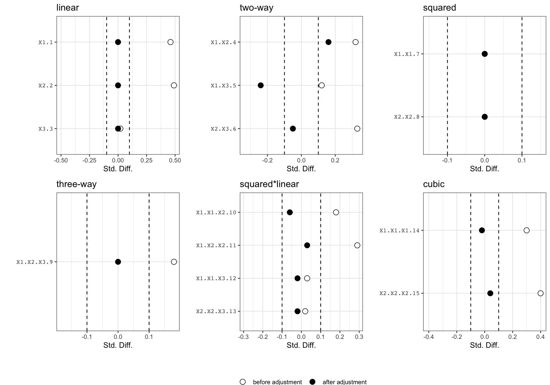
From the above plots, we can see that the linear terms of the covariates are exactly balanced between the treatment and the control groups. We can check the group penalties or penalties applied to each covariate. In this case, the higher-order terms all have relatively high penalties except for two-way interactions, in accordance with the true data generating process.
round(out$group.penalty, 2)
#>         linear        two-way        squared      three-way squared*linear
#>           0.00           5.21           0.00          16.39           4.25
#>          cubic
#>           0.51
round(out$term.penalty, 2)
#>        X1.1        X2.2        X3.3     X1.X2.4     X1.X3.5     X2.X3.6
#>        0.00        0.00        0.00        5.21        5.21        5.21
#>     X1.X1.7     X2.X2.8  X1.X2.X3.9 X1.X1.X2.10 X1.X2.X2.11 X1.X1.X3.12
#>        0.00        0.00       16.39        4.25        4.25        4.25
#> X2.X2.X3.13 X1.X1.X1.14 X2.X2.X2.15
#>        4.25        0.51        0.51
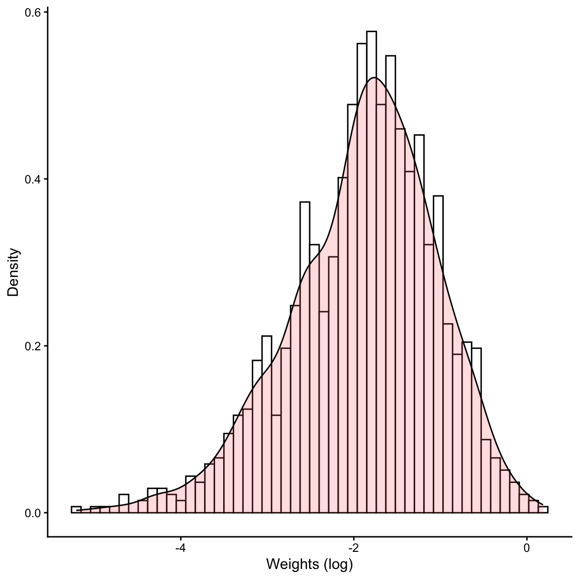
We can also plot the weight distribution for the control units by specifying type = 'weight' in plot(). We can see that the weights are quite concentrated around the unit weight.
plot(out, type='weight')
#> sum(weights) normalized to the number of treated units