# install packages from CRAN
packages <- c("dplyr", "panelView", "ggplot2") # Removed HonestDiD, doParallel
install.packages(setdiff(packages, rownames(installed.packages())))

# install most up-to-date "fect" from Github
if ("fect" %in% rownames(installed.packages()) == FALSE) {
  devtools:: install_github("xuyiqing/fect")
}

# install forked "HonestDiD" package compatible with "fect"
if ("HonestDiDFEct" %in% rownames(installed.packages()) == FALSE) {
  devtools:: install_github("lzy318/HonestDiDFEct") # This is used by fect_sens
}6 Sensitivity Analysis
Download the R code used in this chapter here.
Rambachan and Roth (2023) propose a partial identification approach that relaxes the PT assumption in the post-treatment period by allowing violations that do not exceed the magnitude of those observed in the pre-treatment period. This framework enables sensitivity analysis of estimates from fect or similar methods by comparing pre-treatment deviations from parallel trends (PT) to potential post-treatment deviations.
The key intuition is that if an event study demonstrates strong post-treatment effects yet only minor PT deviations before treatment, any post-treatment departure large enough to reverse these findings must be substantially larger than those observed in the pre-treatment period. Consequently, this approach quantifies how sensitive the estimated dynamic treatment effects are to possible PT violations, using pretrend estimates as the benchmark.
Below, we illustrate how to apply this sensitivity analysis with fect. We focus on two restrictions from Rambachan and Roth (2023): the relative magnitude (RM) restriction and the smoothness restriction, both of which connect pre-treatment PT violations to potential post-treatment counterfactual deviations.
6.1 Install Packages
To begin, you will need to install the necessary packages from CRAN and GitHub.
Load libraries:
6.2 No Treatment Reversals
We begin with an empirical example from Hainmueller and Hangartner (2019), who investigate the effects of indirect democracy versus direct democracy on naturalization rates in Switzerland using municipality-year panel data from 1991 to 2009. The study finds that switching from direct to indirect democracy increased naturalization rates by an average of 1.22 percentage points (Model 1, Table 1).
6.2.1 Implement with Placebo Tests
To implement this method with the imputation estimator, we use the dynamic treatment effects from pre-treatment placebo tests to gauge PT violations and determine whether post-treatment effects remain significant under similar violations. This requires symmetric estimation of dynamic treatment effects in both pre- and post-treatment periods. As (Roth 2024) notes, some estimators (e.g., CSDID without base_period = "universal") may not produce symmetrical estimates.
Below, we designate placebo periods using fect. These placebo periods are excluded during model fitting, and counterfactuals are imputed for both placebo and post-treatment intervals to compute dynamic treatment effects, ensuring consistent estimation across all periods.
By setting placeboTest = TRUE and placebo.period = c(-2, 0), we define three pre-treatment periods as placebo periods. Their dynamic treatment effects serve as the benchmark for PT violations in the post-treatment phase. In the code chunk below, we fit fect with these placebo settings, then use the fect_sens function to perform the sensitivity analysis. This function wraps the procedures from HonestDiDFEct, preparing the output for plotting. Note that not all of Mbarvec, periodMbarvec, Mvec, or periodMvec need to be specified; only the ones you want to use for the sensitivity analysis.
out.fect.placebo <- fect(nat_rate_ord~indirect, data = hh2019,
                         index = c("bfs","year"),
                         method = 'fe', se = TRUE,
                         placeboTest = TRUE, placebo.period = c(-2,0))

# Define post-treatment periods and sensitivity parameters for fect_sens
T.post <- 10 # Number of post-treatment periods based on original analysis
post_periods_vec <- 1:T.post

# Parameters for Relative Magnitude (RM) restriction
Mbar_vec_avg_rm <- seq(0, 1, by = 0.1)    # For average ATT plot
Mbar_vec_period_rm <- c(0, 0.5)          # For period-by-period ATT plot

# Parameters for Smoothness restriction
M_vec_avg_smooth <- seq(0, 0.25, by = 0.05) # For average ATT plot
M_vec_period_smooth <- c(0, 0.1)           # For period-by-period ATT plot

# Run sensitivity analysis using fect_sens
# This function augments out.fect.placebo with sensitivity results
out.fect.placebo <- fect_sens(
  fect.out      = out.fect.placebo,
  post.periods  = post_periods_vec,
  Mbarvec       = Mbar_vec_avg_rm,
  periodMbarvec = Mbar_vec_period_rm,
  Mvec          = M_vec_avg_smooth,
  periodMvec    = M_vec_period_smooth,
  parallel      = TRUE # Set to TRUE for parallel processing if desired
)
6.2.2 RM Restriction
We first explore the Relative Magnitude (RM) restriction. Let \(\delta\) represent potential PT violations for placebo and post-treatment periods. Unlike a standard event study that assumes \(\delta_t=0\) for \(t>0\), RM allows PT deviations as long as they do not exceed \(\bar{M}\) times the maximum deviation between consecutive placebo periods.
The fect package, through fect_sens, utilizes a forked version of HonestDiD, called HonestDiDFEct, which is adapted for fect’s output structure. The RM restriction is defined as:
\[ \Delta^{RM}(\bar{M}) = \left\{\delta : \forall t \geq 0,\; \bigl|\delta_{t+1} - \delta_t\bigr| \leq \bar{M}\cdot\max\bigl( |\delta_{-1} - \delta_{-2}|,\,|\delta_0 - \delta_{-1}| \bigr)\right\}. \]
Here, \(max(|\delta_{-1}-\delta_{-2}|,|\delta_0-\delta_{-1}|)\) matches the largest consecutive discrepancy among the placebo periods. When \(\bar{M}=0\), the PT violation observed at \(t=0\) persists without change into the post-treatment window. Allowing \(\bar{M}>0\) permits \(\delta_t\) to vary across post-treatment periods, but the incremental changes must remain within \(\bar{M}\) times the largest consecutive deviation among placebo periods.
Robust Confidence Set for the ATT
We begin by constructing a robust confidence set for the overall ATT. The fect_sens function has already computed these results, using count-based weights for the ATT by default. We specified Mbarvec = seq(0, 1, by=0.1) in our call to fect_sens. Increasing \(\bar{M}\) allows proportionally larger PT violations in the post-treatment window. When \(\bar{M}=0\), the resulting confidence set behaves as a “de-biased” interval that corrects post-treatment estimates based on the observed PT violation at \(t=0\).
We can now plot the robust confidence intervals for the ATT using the RM restriction with plot() and type = "sens":
plot(out.fect.placebo,
     type = "sens",
     restrict = "rm",
     main = "Relative Magnitude Restriction")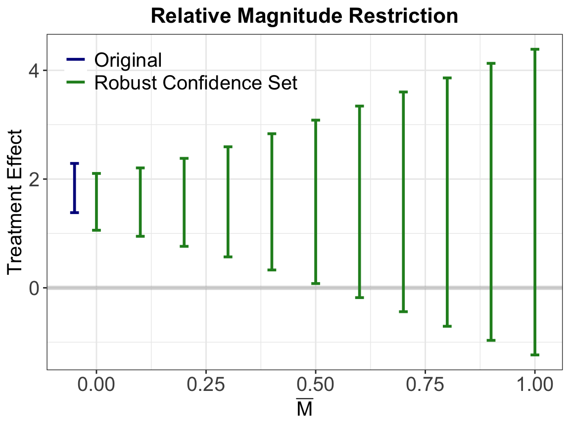
If the robust confidence set excludes zero at \(\bar{M}=0.4\) but includes zero at \(\bar{M}=0.5\), we infer that post-treatment PT violations must be at least half of the maximum observed placebo violation to overturn the estimated effect.
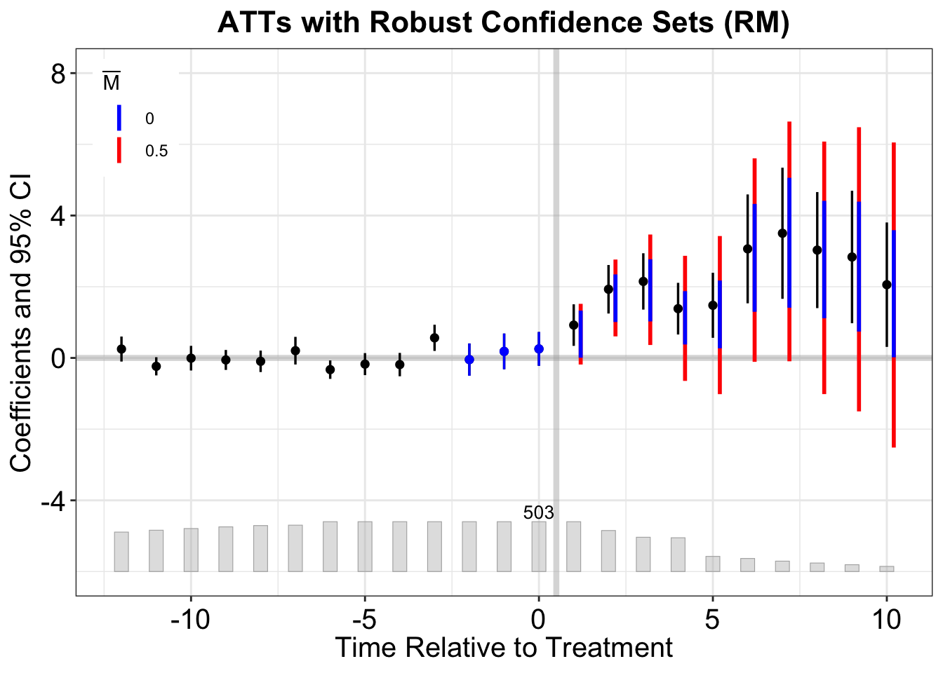
Period-by-Period Robust Confidence Set
The fect_sens function, with the periodMbarvec argument set to c(0, 0.5), computes period-specific robust confidence intervals. We can visualize them using plot() with type = "sens_es":
plot(out.fect.placebo,
    type = "sens_es",
    restrict = "rm",
    main = "ATTs with Robust Confidence Sets (RM)",
    ylab = "Coefficients and 95% CI",
    xlim = c(-12,10),
    ylim = c(-6,8),
    show.count = TRUE)
In the figure, different lines/bands represent the robust confidence intervals for \(\bar{M}=0\) and \(\bar{M}=0.5\). The interval for \(\bar{M}=0\) treats the observed violation at \(t=0\) as persisting into all post-treatment periods, whereas the interval for \(\bar{M}=0.5\) allows added PT violations up to half of the largest placebo discrepancy. These are compared against the original confidence intervals. You can also change the colors using the sens.colors argument in the plot() function. This works for the regular type = "sens" plot as well, but with a vector of only one color.
6.2.3 Smoothness Restriction
A second approach to bounding PT violations is the smoothness restriction, which prevents the post-treatment violation from diverging too sharply from a linear extrapolation of the pre-trend. This restriction is particularly relevant if we suspect a gradually varying or near-linear trend in the potential violation.
Formally, one assumes \(\delta\in\Delta^{SD}(M)\) where
\[ \Delta^{SD}(M) := \bigl\{\delta : \bigl| (\delta_{t+1}-\delta_t) - (\delta_t -\delta_{t-1}) \bigr| \leqslant M,\ \forall t\bigr\}. \]
The parameter \(M\geq 0\) controls how quickly the slope of \(\delta\) can vary. Note that \(M=0\) restricts \(\delta\) to be strictly linear, which does not imply \(\delta=0\).
The fect_sens function, using the Mvec argument (set to seq(0,0.25,0.05) in our call), has already computed these results. We plot them for the overall ATT using plot() with type = "sens" and restrict = "sm":
plot(out.fect.placebo,
    type = "sens",
    restrict = "sm",
    main = "Smoothness Restriction")
Here, if the post-treatment effect is indistinguishable from zero even when \(M=0\), it suggests that the estimated average treatment effect may not be robust to a strictly linear violation of PT observed in the placebo periods, let alone to variations in the slope of this linear trend.
Period-by-Period Robust Confidence Set
Finally, we construct period-specific robust confidence sets under the smoothness restriction. The fect_sens function, with periodMvec set to c(0, 0.1) in our call, calculates these. The plot is generated using type = "sens_es" and restrict = "sm":
plot(out.fect.placebo,
    type = "sens_es",
    restrict = "sm",
    main = "ATTs with Robust Confidence Sets (Smoothness)",
    ylab = "Coefficients and 95% CI",
    xlim = c(-12,10), # Adjusted to match original detailed plot
    ylim = c(-12,15),
    show.count = TRUE)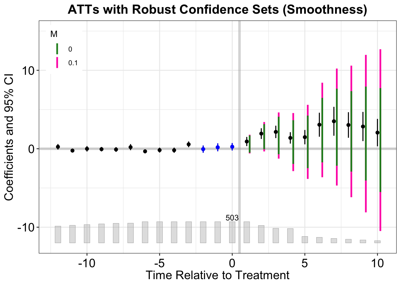
In this figure, different lines/bands will represent the robust CIs for \(M=0\) (strictly linear PT violation) and \(M=0.1\) (allowing a slope deviation of 0.1). These are compared against the original estimates and placebo period estimates to assess the robustness of dynamic treatment effects.
6.3 How to Cite
Please cite Rambachan and Roth (2023) for their original contribution to the sensitivity analysis framework for causal panel analysis. If you find this tutorial helpful, you can cite Chiu et al. (2025).