# install packages from CRAN
packages <- c("dplyr", "fixest", "did", "didimputation",
              "panelView", "ggplot2", "bacondecomp", "HonestDiD",
              "DIDmultiplegtDYN", "PanelMatch", "readstata13")
install.packages(setdiff(packages, rownames(installed.packages())))

# install most up-to-date "fect" from Github
if ("fect" %in% rownames(installed.packages()) == FALSE) {
  devtools:: install_github("xuyiqing/fect")
}

# install forked "HonestDiD" package compatible with "fect"
if ("HonestDiDFEct" %in% rownames(installed.packages()) == FALSE) {
  devtools:: install_github("lzy318/HonestDiDFEct")
}5 New DID Methods
This chapter, authored by Ziyi Liu and Yiqing Xu, complements Chiu et al. (2025) (paper, slides). Rivka Lipkovitz also contributes to this tutorial. Download the R code used in this chapter here.
In recent years, researchers have proposed various heterogeneous treatment effect (HTE) robust estimators for causal panel analysis under parallel trends (PT) as alternatives to traditional two-way fixed effects (TWFE) models. Examples include those proposed by Cengiz et al. (2019), Sun and Abraham (2021), Callaway and Sant’Anna (2021), Chaisemartin and D’Haultfœuille (2020), Imai, Kim, and Wang (2023), Borusyak, Jaravel, and Spiess (2024), and Liu, Wang, and Xu (2024). These methods are closely connected to the classic difference-in-differences (DID) estimator.
This chapter will guide you through implementing these HTE-robust estimators, as well as TWFE, in R. It will also provide instructions on creating event study plots to display estimated dynamic treatment effects. In the process, we will present a recommended pipeline for analyzing panel data, covering data exploration, estimation, result visualization, and diagnostic tests.
We illustrate these methods with two empirical examples: Hainmueller and Hangartner (2019) (without treatment reversals) and Grumbach and Sahn (2020) (with treatment reversals).
5.1 Install Packages
To begin, you will need to install the necessary packages from CRAN and GitHub.
Load libraries:
library(dplyr)
library(readstata13)
library(fixest)
library(did)
library(fect)
library(panelView)
library(PanelMatch)
library(ggplot2)
library(bacondecomp)
library(fect)
library(didimputation)
library(doParallel)
library(HonestDiD)
library(HonestDiDFEct)
library(DIDmultiplegtDYN) # may require XQuartz
5.2 No Treatment Reversals
We begin with an empirical example from Hainmueller and Hangartner (2019), who investigate the effects of indirect democracy versus direct democracy on naturalization rates in Switzerland using municipality-year panel data from 1991 to 2009. The study finds that switching from direct to indirect democracy increased naturalization rates by an average of 1.22 percentage points (Model 1, Table 1).
5.2.1 Visualizing Data
First, we examine the evolution of treatment status using the panelView package. The variables bfs and year represent the unit and time indicators, respectively. The treatment variable is indirect, and the outcome is nat_rate_ord. In the baseline analysis, we exclude covariates. We set by.timing = TRUE to sort units by the timing of treatment receipt.
panelview(nat_rate_ord ~ indirect, data = data, index = c("bfs","year"),
  xlab = "Year", ylab = "Unit", display.all = T,
  gridOff = TRUE, by.timing = TRUE)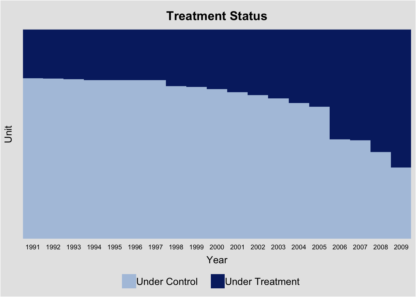
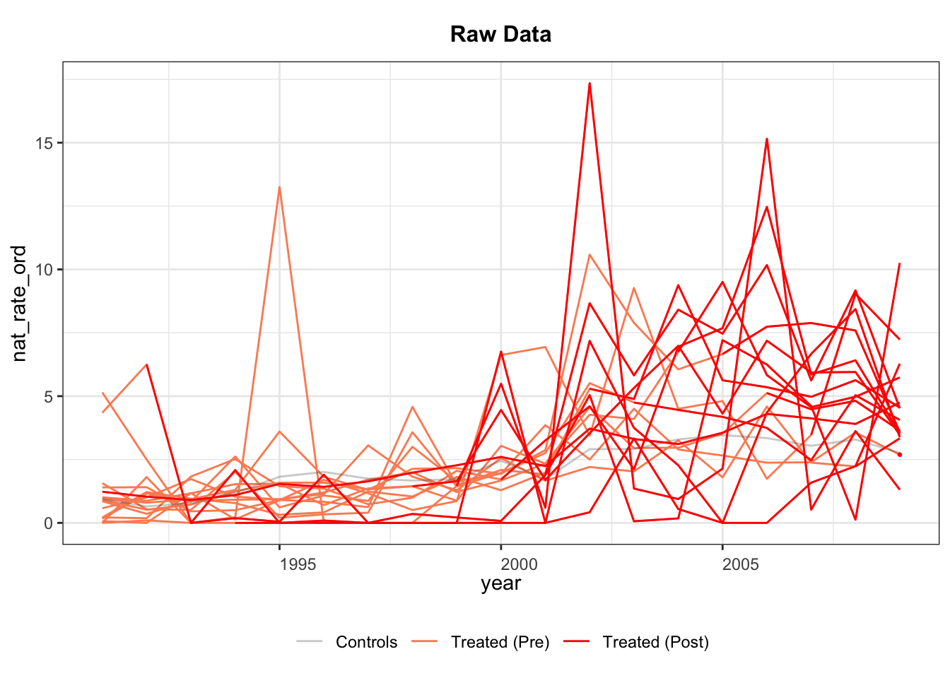
The treatment status plot shows that treatment is introduced in different years across municipalities, with no treatment reversals (a staggered adoption setting). Following Sun and Abraham (2021), we define units that receive treatment in the same year as a cohort. We can then use panelView to plot the average outcomes for each cohort. Because there are many cohorts, the figure is not as informative as desired.
5.2.2 TWFE
The staggered adoption setup allows us to implement several estimators to obtain the treatment effect estimates. We will first estimate a two-way fixed-effects (TWFE) model, as the authors do in the paper: \[Y_{it} = \alpha_i + \xi_t + \delta^{TWFE}D_{it} + \epsilon\] We can implement this estimator using thefeols function in the fixest package. The estimated coefficient using TWFE is 1.339, with a standard error of 0.187.
# remember to cluster standard errors
model.twfe.0 <- feols(nat_rate_ord~indirect|bfs+year,
                      data=data, cluster = "bfs")
print(model.twfe.0)
#> OLS estimation, Dep. Var.: nat_rate_ord
#> Observations: 22,971
#> Fixed-effects: bfs: 1,209,  year: 19
#> Standard-errors: Clustered (bfs)
#>          Estimate Std. Error t value   Pr(>|t|)
#> indirect  1.33932   0.186525 7.18039 1.2117e-12 ***
#> ---
#> Signif. codes:  0 '***' 0.001 '**' 0.01 '*' 0.05 '.' 0.1 ' ' 1
#> RMSE: 4.09541     Adj. R2: 0.152719
#>                 Within R2: 0.005173
5.2.3 Goodman-Bacon Decomposition
Goodman-Bacon (2021) shows that the TWFE estimator in a staggered adoption setting can be expressed as a weighted average of all possible 2×2 DID estimates across different cohorts. However, when treatment effects vary over time across cohorts, forbidden comparisons—where post-treatment data from early adopters serve as controls for late adopters—can introduce bias into the TWFE estimator. To address this, we follow the procedure in Goodman-Bacon (2021) and decompose the TWFE estimate using the bacon function from the bacondecomp package.
data.complete <- data[which(!is.na(data$nat_rate_ord)),] # bacon requires no missingness in the data
df_bacon <- bacon(nat_rate_ord~indirect,
                  data = data.complete,
                  id_var = "bfs",
                  time_var = "year")
#>                       type  weight avg_est
#> 1 Earlier vs Later Treated 0.17605 1.97771
#> 2  Later vs Always Treated 0.31446 0.75233
#> 3 Later vs Earlier Treated 0.05170 0.32310
#> 4     Treated vs Untreated 0.45779 1.61180
ggplot(df_bacon) +
   aes(x = weight, y = estimate, shape = factor(type), color = factor(type)) +
   labs(x = "Weight", y = "Estimate", shape = "Type", color = 'Type') +
   geom_point()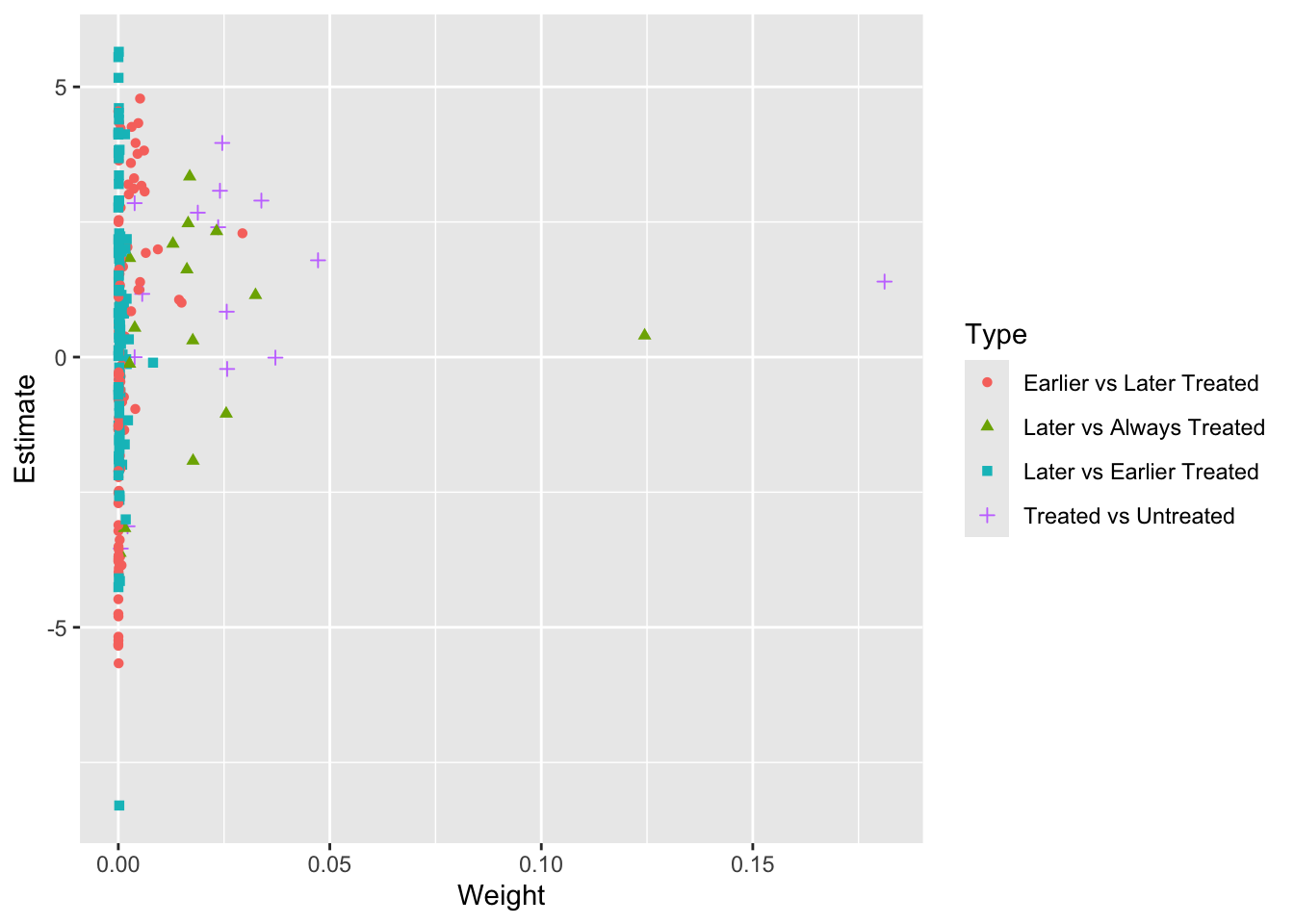
The decomposition of the TWFE estimator in a staggered adoption setting, as shown by Goodman-Bacon (2021), reveals that the largest contribution to the TWFE estimate comes from DIDs comparing ever-treated cohorts switching into treatment with the never-treated (purple crosses labeled “Treated vs Untreated”). The second-largest contribution comes from DIDs comparing ever-treated cohorts switching into treatment with other ever-treated cohorts still in their pretreatment periods (red dots labeled “Earlier vs Later Treated”), followed by forbidden comparisons between ever-treated cohorts and the always-treated (green triangles labeled “Later vs Always Treated”). The smallest contribution comes from “forbidden” DIDs comparing ever-treated cohorts switching into treatment with other ever-treated cohorts already treated (blue squares labeled “Later vs Earlier Treated”).
Before applying HTE-robust estimators, we first remove the always-treated units for easier comparison. Then, we create an event study plot using a dynamic specification of TWFE.
# drop always treated units
df <- as.data.frame(data %>%
                      group_by(bfs) %>%
                      mutate(treatment_mean = mean(indirect,na.rm = TRUE)))
df.use <- df[which(df$treatment_mean<1),]

# Re-estimate TWFE on this Sub-sample
model.twfe.1 <- feols(nat_rate_ord~indirect|bfs+year,
                      data=df.use, cluster = "bfs")
print(model.twfe.1)
#> OLS estimation, Dep. Var.: nat_rate_ord
#> Observations: 17,594
#> Fixed-effects: bfs: 926,  year: 19
#> Standard-errors: Clustered (bfs)
#>          Estimate Std. Error t value  Pr(>|t|)
#> indirect  1.60858   0.195296 8.23661 6.009e-16 ***
#> ---
#> Signif. codes:  0 '***' 0.001 '**' 0.01 '*' 0.05 '.' 0.1 ' ' 1
#> RMSE: 4.43613     Adj. R2: 0.143692
#>                 Within R2: 0.007415
After removing the always-treated units, the estimated treatment effect increases to 1.609, with a standard error of 0.195.
5.2.4 TWFE Event Study Plot
To create an event study plot, we first generate the cohort index and the relative time period for each observation in relation to treatment. These details are essential for various HTE-robust estimators, such as those in Sun and Abraham (2021) and Callaway and Sant’Anna (2021). We use the get.cohort function in fect to generate these indices. To maintain consistency with canonical TWFE regressions, we set start0 = TRUE, designating period 0 as the first post-treatment period and period -1 as the last pre-treatment period.
df.use <- get.cohort(df.use, D = "indirect", index=c("bfs","year"),
                     start0 = TRUE)
head(df.use[,-5],19)
#>    bfs year nat_rate_ord indirect FirstTreat      Cohort Time_to_Treatment
#> 1    1 1991     0.000000        0       2006 Cohort:2006               -15
#> 2    1 1992     0.000000        0       2006 Cohort:2006               -14
#> 3    1 1993     0.000000        0       2006 Cohort:2006               -13
#> 4    1 1994     3.448276        0       2006 Cohort:2006               -12
#> 5    1 1995     0.000000        0       2006 Cohort:2006               -11
#> 6    1 1996     0.000000        0       2006 Cohort:2006               -10
#> 7    1 1997     0.000000        0       2006 Cohort:2006                -9
#> 8    1 1998     0.000000        0       2006 Cohort:2006                -8
#> 9    1 1999     0.000000        0       2006 Cohort:2006                -7
#> 10   1 2000     0.000000        0       2006 Cohort:2006                -6
#> 11   1 2001     2.380952        0       2006 Cohort:2006                -5
#> 12   1 2002     0.000000        0       2006 Cohort:2006                -4
#> 13   1 2003     0.000000        0       2006 Cohort:2006                -3
#> 14   1 2004     0.000000        0       2006 Cohort:2006                -2
#> 15   1 2005     0.000000        0       2006 Cohort:2006                -1
#> 16   1 2006     1.612903        1       2006 Cohort:2006                 0
#> 17   1 2007    10.937500        1       2006 Cohort:2006                 1
#> 18   1 2008    14.285715        1       2006 Cohort:2006                 2
#> 19   1 2009     9.677419        1       2006 Cohort:2006                 3
The column FirstTreat indicates the first period when a unit receives treatment (set to NA for never-treated units). The column Time_to_Treatment represents the relative period to treatment onset (set to NA for always-treated and never-treated units). The period -1 corresponds to the last pre-treatment period.
Now, we run a dynamic TWFE regression, also known as a model with “leads and lags.” This is the standard approach for estimating dynamic treatment effects in event studies. The model includes a series of interaction terms between a dummy indicating whether a unit is treated and each lead and lag indicator relative to treatment in a TWFE regression. This specification allows effects to vary over time, typically using the period immediately before treatment as the reference period. If the regression is fully saturated and there is no HTE across cohorts, the dynamic TWFE model can consistently estimate the dynamic treatment effect.
We use feols to implement this estimator. The column Time_to_Treatment can serve as the lead/lag indicator (we need to replace the NA in Time_to_Treatment with an arbitrary number). Note that the period -1 in Time_to_Treatment corresponds to the last pre-treatment period and is the reference period.
# Dynamic TWFE
df.twfe <- df.use
# drop always treated units
df.twfe$treat <- as.numeric(df.twfe$treatment_mean>0)
df.twfe[which(is.na(df.twfe$Time_to_Treatment)),'Time_to_Treatment'] <- 0 # can be an arbitrary value
twfe.est <- feols(nat_rate_ord ~ i(Time_to_Treatment, treat, ref = -1)| bfs + year,
data = df.twfe, cluster = "bfs")
twfe.output <- as.matrix(twfe.est$coeftable)
print(round(twfe.output, 3))
#> Estimate Std. Error t value Pr(>|t|)
#> Time_to_Treatment::-18:treat -0.321 0.633 -0.507 0.612
#> Time_to_Treatment::-17:treat -0.119 0.391 -0.303 0.762
#> Time_to_Treatment::-16:treat -0.396 0.403 -0.982 0.326
#> Time_to_Treatment::-15:treat -0.411 0.344 -1.195 0.232
#> Time_to_Treatment::-14:treat 0.245 0.369 0.662 0.508
#> Time_to_Treatment::-13:treat -0.044 0.354 -0.125 0.900
#> Time_to_Treatment::-12:treat -0.546 0.315 -1.732 0.084
#> Time_to_Treatment::-11:treat -0.293 0.347 -0.845 0.398
#> Time_to_Treatment::-10:treat -0.424 0.319 -1.328 0.185
#> Time_to_Treatment::-9:treat -0.467 0.301 -1.552 0.121
#> Time_to_Treatment::-8:treat -0.116 0.334 -0.347 0.729
#> Time_to_Treatment::-7:treat -0.724 0.306 -2.369 0.018
#> Time_to_Treatment::-6:treat -0.573 0.317 -1.807 0.071
#> Time_to_Treatment::-5:treat -0.555 0.309 -1.795 0.073
#> Time_to_Treatment::-4:treat 0.066 0.345 0.192 0.848
#> Time_to_Treatment::-3:treat -0.510 0.316 -1.611 0.108
#> Time_to_Treatment::-2:treat -0.195 0.330 -0.591 0.555
#> Time_to_Treatment::0:treat 0.523 0.360 1.453 0.146
#> Time_to_Treatment::1:treat 1.669 0.368 4.536 0.000
#> Time_to_Treatment::2:treat 1.724 0.471 3.658 0.000
#> Time_to_Treatment::3:treat 1.178 0.401 2.942 0.003
#> Time_to_Treatment::4:treat 0.756 0.479 1.580 0.114
#> Time_to_Treatment::5:treat 2.438 0.705 3.456 0.001
#> Time_to_Treatment::6:treat 2.849 0.805 3.537 0.000
#> Time_to_Treatment::7:treat 2.409 0.784 3.074 0.002
#> Time_to_Treatment::8:treat 2.270 0.798 2.846 0.005
#> Time_to_Treatment::9:treat 2.393 0.863 2.772 0.006
#> Time_to_Treatment::10:treat 2.003 0.954 2.100 0.036
#> Time_to_Treatment::11:treat 0.843 0.560 1.504 0.133
#> Time_to_Treatment::12:treat 3.832 2.300 1.666 0.096
#> Time_to_Treatment::13:treat 4.436 2.322 1.910 0.056
#> Time_to_Treatment::14:treat 4.757 3.486 1.365 0.173
#> Time_to_Treatment::15:treat 1.542 1.415 1.090 0.276
#> Time_to_Treatment::16:treat 7.169 4.844 1.480 0.139
#> Time_to_Treatment::17:treat 6.491 2.727 2.381 0.017
#> attr(,"type")
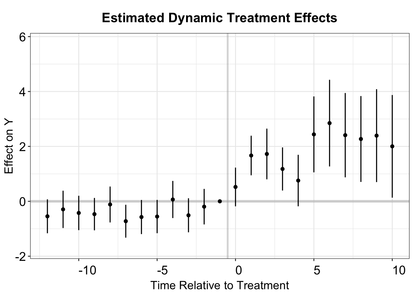
#> [1] "Clustered (bfs)"fect includes a plotting function, esplot(), to create an event study plot based on a vector of point estimates and estimated standard errors. Here, we use this function to examine dynamic effects over a 13-period pre-treatment span and a 10-period post-treatment span. The data reveals a significant treatment effect, along with a subtle pre-trend discrepancy in several periods preceding treatment. Notably, esplot() treats period 0 as the last pre-treatment period by default, so the period index must be shifted by one.
twfe.output <- as.data.frame(twfe.output)
twfe.output$Time <- c(c(-18:-2),c(0:17))+1
p.twfe <- esplot(twfe.output,Period = 'Time',Estimate = 'Estimate',
                               SE = 'Std. Error', xlim = c(-12,10))
p.twfe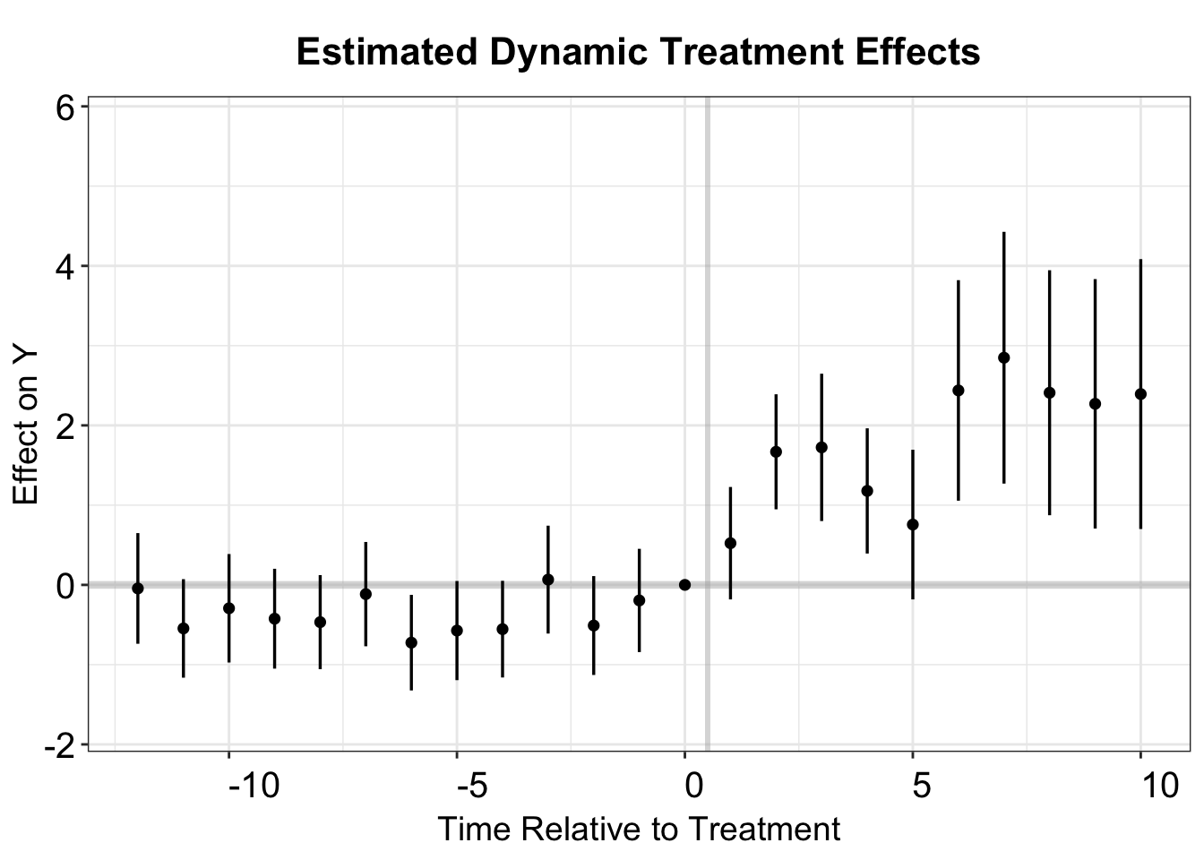
By setting start0 = TRUE, we designate period 0 as the first post-treatment period, making period -1 the last pre-treatment period. As a result, there is no need to shift the period index, as it already aligns with the conventional TWFE framework.
5.2.5 Stacked DID
Cengiz et al. (2019) examine the effect of variations in minimum wage on low-wage employment across 138 state-level minimum wage changes in the United States between 1979 and 2016, using a stacked DID approach. A similar estimator is also implemented in the Stata package STACKEDEV (Bleiberg 2021). See a simple illustration below.

The stacked DID method removes the bias caused by forbidden comparisons in the Goodman-Bacon decomposition. However, it returns a variance-weighted ATT with the implicit weights chosen by OLS instead of the ATT.
df.st <- NULL
target.cohorts <- setdiff(unique(df.use$Cohort),"Control")
k <- 1
for(cohort in target.cohorts){
  df.sub <- df.use[which(df.use$Cohort%in%c(cohort,"Control")),]
  df.sub$stack <- k
  df.st <- rbind(df.st,df.sub)
  k <- k + 1
}
df.st$st_unit <- as.numeric(factor(paste0(df.st$stack,'-',df.st$bfs)))
df.st$st_year <- as.numeric(factor(paste0(df.st$stack,'-',df.st$year)))
model.st <- feols(nat_rate_ord~indirect|st_unit+st_year,
                  data=df.st, cluster = "st_unit")

print(model.st)
#> OLS estimation, Dep. Var.: nat_rate_ord
#> Observations: 127,186
#> Fixed-effects: st_unit: 6,694,  st_year: 285
#> Standard-errors: Clustered (st_unit)
#>          Estimate Std. Error t value  Pr(>|t|)
#> indirect  1.66861    0.18237 9.14958 < 2.2e-16 ***
#> ---
#> Signif. codes:  0 '***' 0.001 '**' 0.01 '*' 0.05 '.' 0.1 ' ' 1
#> RMSE: 3.9095     Adj. R2: 0.130512
#>                Within R2: 0.001783
We then make an event study plot using a dynamic specification.
df.st$treat <- as.numeric(df.st$treatment_mean>0)
df.st[which(is.na(df.st$Time_to_Treatment)),'Time_to_Treatment'] <- 1000
# note, this "1000" can be arbitrary value

st.est <- feols(nat_rate_ord ~
                  i(Time_to_Treatment, treat, ref = -1)| st_unit +
                  st_year,data = df.st,cluster = "st_unit")

# make plot
st.output <- as.data.frame(st.est$coeftable)
st.output$Time <- c(c(-18:-2),c(0:17))+1
p.st <- esplot(st.output,Period = 'Time',Estimate = 'Estimate',
                               SE = 'Std. Error', xlim = c(-12,10))
p.st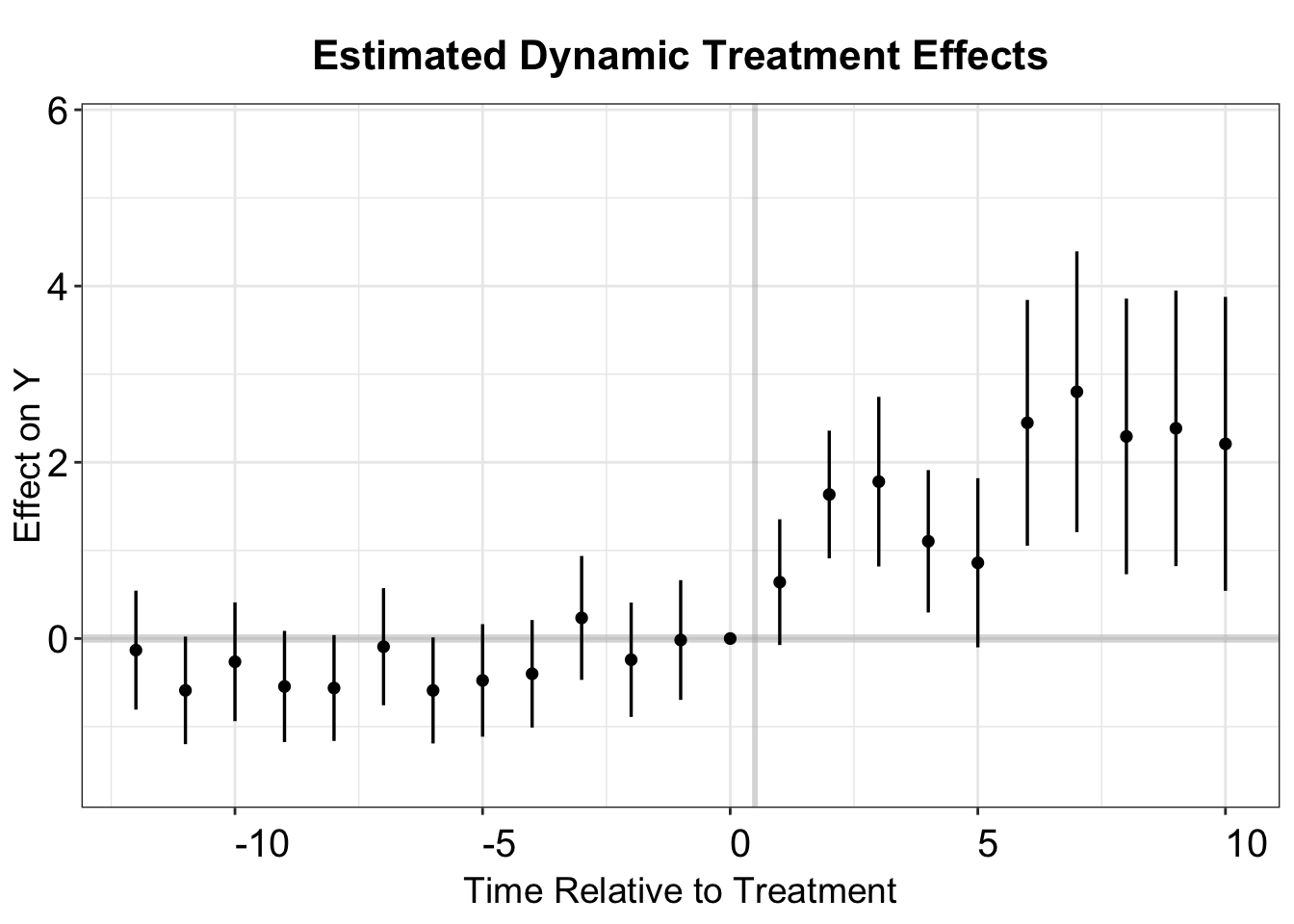
The stacked DID plot closely resembles that of the TWFE model, suggesting that potential bias from forbidden comparisons is minimal.
5.2.6 Interaction Weighted
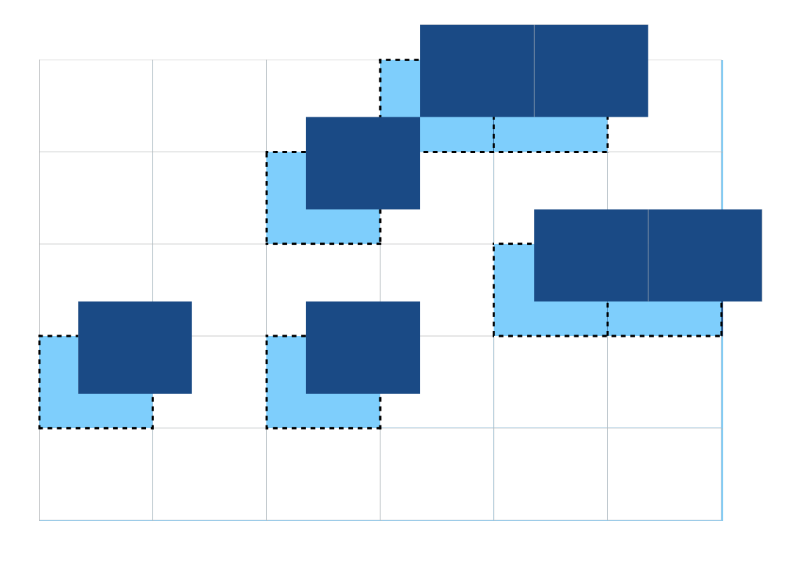
Sun and Abraham (2021) proposes an interaction-weighted (IW) estimator for estimating the ATT. the IW estimator computes a weighted average of ATT estimates for each cohort, obtained from a TWFE regression where cohort dummies are fully interacted with indicators of relative time to treatment onset. See a simple illustration below.
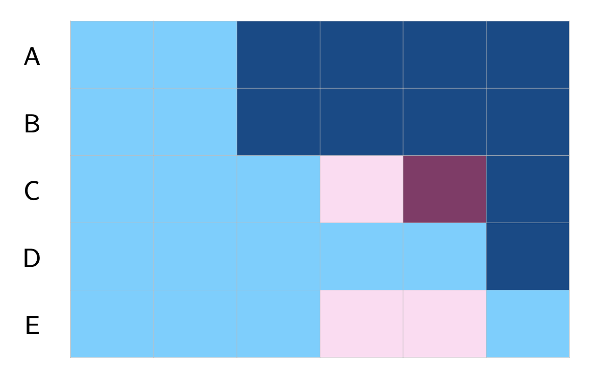
The IW estimator is HTE-robust and can be implemented using the sunab function in the fixest package. The column FirstTreat serves as the cohort indicator, with any missing values replaced by an arbitrary number. The estimated ATT using the IW estimator is 1.331, with a standard error of 0.288.
df.sa <- df.use
df.sa[which(is.na(df.sa$FirstTreat)),"FirstTreat"] <- 1000
# above, replace NA with an arbitrary number

model.sa.1 <- feols(nat_rate_ord~sunab(FirstTreat,year)|bfs+year,
                    data = df.sa, cluster = "bfs")
summary(model.sa.1,agg = "ATT")
#> OLS estimation, Dep. Var.: nat_rate_ord
#> Observations: 17,594
#> Fixed-effects: bfs: 926,  year: 19
#> Standard-errors: Clustered (bfs)
#>     Estimate Std. Error t value   Pr(>|t|)
#> ATT   1.3309   0.287971 4.62163 4.3474e-06 ***
#> ---
#> Signif. codes:  0 '***' 0.001 '**' 0.01 '*' 0.05 '.' 0.1 ' ' 1
#> RMSE: 4.34795     Adj. R2: 0.163888
#>                 Within R2: 0.046484
The estimation results are saved coeftable for plotting. We can make an event study plot as before. The results are quite similar to TWFE and stacked DID.

5.2.7 CSDID
Callaway and Sant’Anna (2021) propose a doubly robust estimator, known as CSDID, which incorporates pre-treatment covariates by using either never-treated or not-yet-treated units as the comparison group. Due to lack of time-invariant covariates, we use only the outcome model (rather than the full doubly robust estimator) to estimate the ATT and dynamic treatment effects.
First, we use the never-treated units as the comparison group. The column FirstTreat serves as the cohort indicator, with missing values replaced by 0. The estimated ATT is numerically identical to the IW estimator. Additionally, we set bstrap = FALSE to report the analytical standard error, which is 0.302.
df.cs <- df.use
df.cs[which(is.na(df.cs$FirstTreat)),"FirstTreat"] <- 0 # replace NA with 0
cs.est.1 <- att_gt(yname = "nat_rate_ord",
                 gname = "FirstTreat",
                 idname = "bfs",
                 tname = "year",
                 xformla = ~1,
                 control_group = "nevertreated",
                 allow_unbalanced_panel = TRUE,
                 data = df.cs,
                 est_method = "reg")
cs.est.att.1 <- aggte(cs.est.1, type = "simple", na.rm=T, bstrap = F)
print(cs.est.att.1)
#>
#> Call:
#> aggte(MP = cs.est.1, type = "simple", na.rm = T, bstrap = F)
#>
#> Reference: Callaway, Brantly and Pedro H.C. Sant'Anna.  "Difference-in-Differences with Multiple Time Periods." Journal of Econometrics, Vol. 225, No. 2, pp. 200-230, 2021. <https://doi.org/10.1016/j.jeconom.2020.12.001>, <https://arxiv.org/abs/1803.09015>
#>
#>
#>     ATT    Std. Error     [ 95%  Conf. Int.]
#>  1.3309        0.3019     0.7392      1.9226 *
#>
#>
#> ---
#> Signif. codes: `*' confidence band does not cover 0
#>
#> Control Group:  Never Treated,  Anticipation Periods:  0
#> Estimation Method:  Outcome Regression
Using the csdid package, we can use the aggte function to aggregate cohort-period average treatment effects. We set bstrap = FALSE to report analytical standard errors and cband = FALSE to display period-wise confidence intervals, allowing for easy comparison with other estimators. While aggte can compute uniform confidence bands by setting both cband and bstrap to TRUE, we opt to report period-wise intervals in this case.
cs.att.1 <- aggte(cs.est.1, type = "dynamic",
                  bstrap=FALSE, cband=FALSE, na.rm=T)
print(cs.att.1)
#>
#> Call:
#> aggte(MP = cs.est.1, type = "dynamic", na.rm = T, bstrap = FALSE,
#>     cband = FALSE)
#>
#> Reference: Callaway, Brantly and Pedro H.C. Sant'Anna.  "Difference-in-Differences with Multiple Time Periods." Journal of Econometrics, Vol. 225, No. 2, pp. 200-230, 2021. <https://doi.org/10.1016/j.jeconom.2020.12.001>, <https://arxiv.org/abs/1803.09015>
#>
#>
#> Overall summary of ATT's based on event-study/dynamic aggregation:
#>     ATT    Std. Error     [ 95%  Conf. Int.]
#>  1.2205        0.6314    -0.0171       2.458
#>
#>
#> Dynamic Effects:
#>  Event time Estimate Std. Error [95% Pointwise  Conf. Band]
#>         -17   0.1350     0.6467         -1.1324      1.4025
#>         -16  -0.0839     0.3583         -0.7861      0.6183
#>         -15   0.1467     0.3964         -0.6303      0.9236
#>         -14   0.7509     0.3219          0.1200      1.3818 *
#>         -13  -0.2318     0.3392         -0.8967      0.4331
#>         -12  -0.5851     0.2814         -1.1367     -0.0335 *
#>         -11   0.2656     0.2705         -0.2647      0.7958
#>         -10  -0.2386     0.2805         -0.7883      0.3111
#>          -9   0.0576     0.2702         -0.4721      0.5872
#>          -8   0.5244     0.3165         -0.0959      1.1448
#>          -7  -0.6282     0.3132         -1.2420     -0.0144 *
#>          -6   0.1081     0.2565         -0.3946      0.6108
#>          -5   0.1623     0.2890         -0.4041      0.7287
#>          -4   0.6485     0.3380         -0.0139      1.3109
#>          -3  -0.6161     0.3674         -1.3362      0.1040
#>          -2   0.1505     0.3355         -0.5071      0.8081
#>          -1   0.0279     0.3425         -0.6435      0.6992
#>           0   0.7141     0.3754         -0.0217      1.4500
#>           1   1.5846     0.3681          0.8632      2.3060 *
#>           2   1.6337     0.5118          0.6306      2.6369 *
#>           3   0.9090     0.4396          0.0473      1.7707 *
#>           4   0.4091     0.5725         -0.7130      1.5311
#>           5   2.1106     0.7976          0.5473      3.6739 *
#>           6   2.4842     0.9078          0.7051      4.2634 *
#>           7   2.3802     0.8538          0.7068      4.0535 *
#>           8   2.5602     0.8723          0.8506      4.2699 *
#>           9   2.0100     0.9769          0.0953      3.9246 *
#>          10   1.6391     1.0257         -0.3712      3.6494
#>          11   0.0298     0.6100         -1.1658      1.2253
#>          12   0.6942     2.8043         -4.8021      6.1904
#>          13   1.1355     2.3284         -3.4281      5.6991
#>          14   1.3625     3.4131         -5.3270      8.0519
#>          15  -2.0699     1.7160         -5.4331      1.2933
#>          16   2.2743     3.6182         -4.8172      9.3658
#>          17   0.1072     4.5338         -8.7789      8.9934
#> ---
#> Signif. codes: `*' confidence band does not cover 0
#>
#> Control Group:  Never Treated,  Anticipation Periods:  0
#> Estimation Method:  Outcome Regression
The estimated dynamic treatment effects in the post-treatment period are numerically identical to those from the IW estimator. However, pre-treatment estimates may differ because csdid defaults to using the preceding period as the reference point in pre-treatment periods.
cs.output <- cbind.data.frame(Estimate = cs.att.1$att.egt,
                              SE = cs.att.1$se.egt,
                              time = cs.att.1$egt + 1)
p.cs.1 <- esplot(cs.output,Period = 'time',Estimate = 'Estimate',
                               SE = 'SE', xlim = c(-12,10))
p.cs.1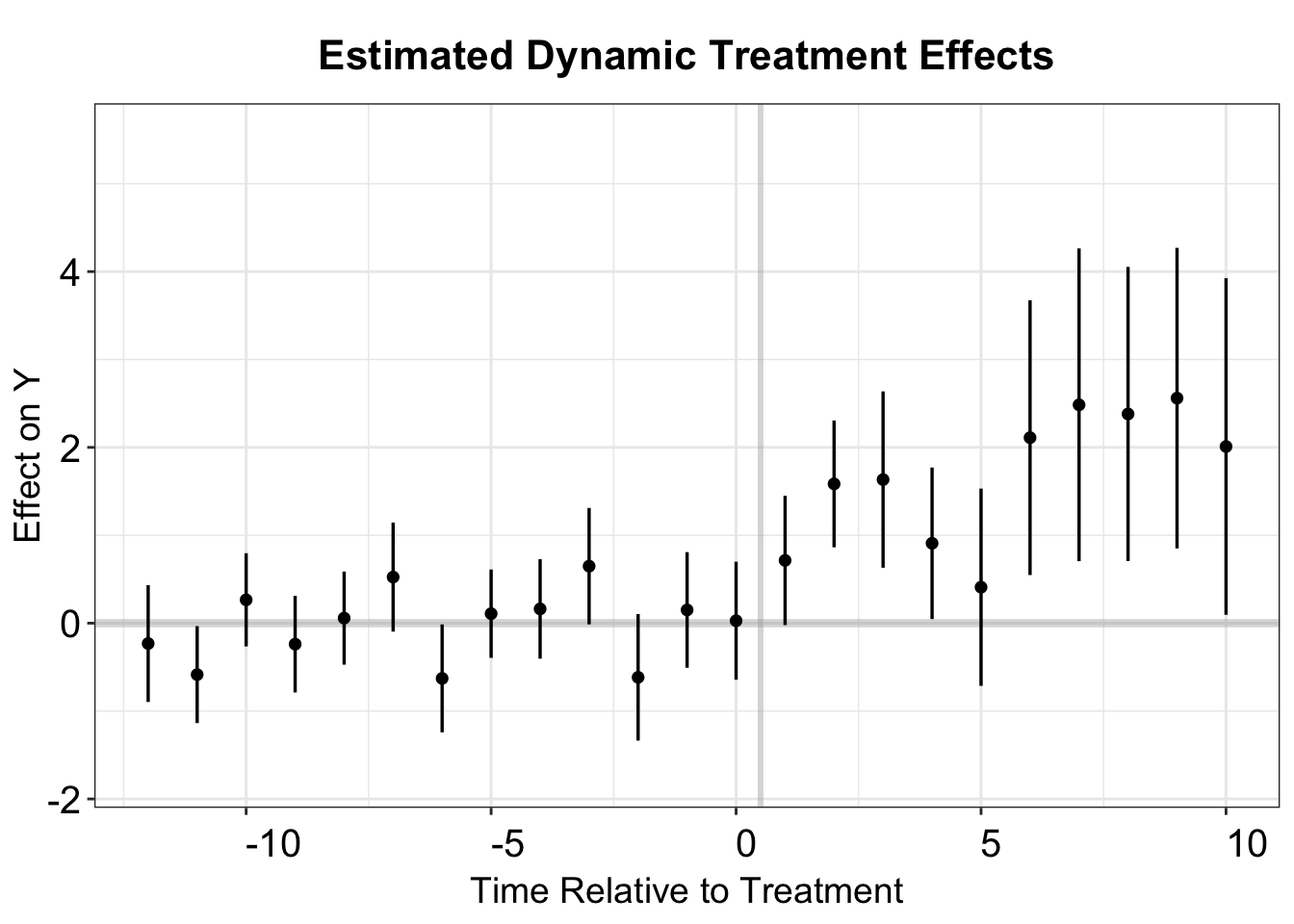
We prefer to set base_period = "universal", which designates the last pre-treatment period as the reference period. This produces results that closely align with the IW estimator.
cs.est.1.u <- att_gt(yname = "nat_rate_ord",
                 gname = "FirstTreat",
                 idname = "bfs",
                 tname = "year",
                 xformla = ~1,
                 control_group = "nevertreated",
                 allow_unbalanced_panel = TRUE,
                 data = df.cs,
                 est_method = "reg",
                 base_period = "universal")
cs.att.1.u <- aggte(cs.est.1.u, type = "dynamic",
                    bstrap=FALSE, cband=FALSE, na.rm=T)
cs.output.u <- cbind.data.frame(Estimate = cs.att.1.u$att.egt,
                                SE = cs.att.1.u$se.egt,
                                time = cs.att.1.u$egt + 1)
p.cs.1.u <- esplot(cs.output.u,Period = 'time',Estimate = 'Estimate',
                               SE = 'SE', xlim = c(-12,10))
p.cs.1.u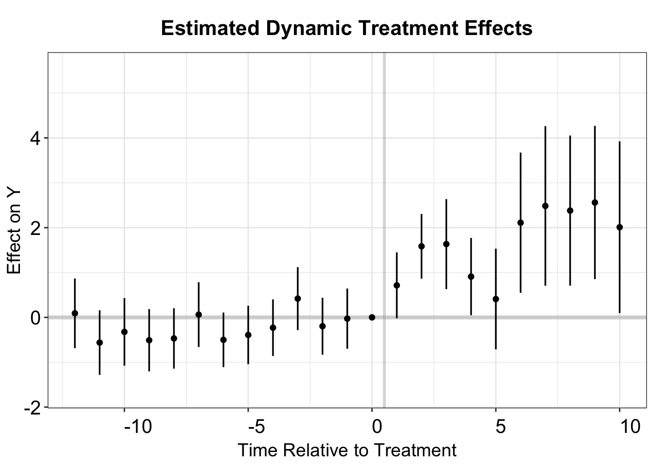
One advantage of CSDID is the ability to use not-yet-treated units as the comparison group by setting control_group = "notyettreated". See a simple illustration below.
The choice of the comparison group depends on the specific version of the parallel trends assumption that researchers aim to justify. The estimated ATT is 1.292, with a standard error of 0.308.
cs.est.2 <- att_gt(yname = "nat_rate_ord",
                   gname = "FirstTreat",
                   idname = "bfs",
                   tname = "year",
                   xformla = ~1,
                   control_group = "notyettreated",
                   allow_unbalanced_panel = TRUE,
                   data = df.cs,
                   est_method = "reg")
cs.est.att.2 <- aggte(cs.est.2, type = "simple",na.rm=T, bstrap = F)
print(cs.est.att.2)
#>
#> Call:
#> aggte(MP = cs.est.2, type = "simple", na.rm = T, bstrap = F)
#>
#> Reference: Callaway, Brantly and Pedro H.C. Sant'Anna.  "Difference-in-Differences with Multiple Time Periods." Journal of Econometrics, Vol. 225, No. 2, pp. 200-230, 2021. <https://doi.org/10.1016/j.jeconom.2020.12.001>, <https://arxiv.org/abs/1803.09015>
#>
#>
#>     ATT    Std. Error     [ 95%  Conf. Int.]
#>  1.2923         0.308     0.6886       1.896 *
#>
#>
#> ---
#> Signif. codes: `*' confidence band does not cover 0
#>
#> Control Group:  Not Yet Treated,  Anticipation Periods:  0
#> Estimation Method:  Outcome Regression
We can calculate the dynamic treatment effects using the same method, and then use esplot to make the event study plot. Note that we set the reference period to be the last pre-treatment period.
cs.est.2.u <- att_gt(yname = "nat_rate_ord", gname = "FirstTreat",
                     idname = "bfs", tname = "year", xformla = ~1,
                     control_group = "notyettreated",
                     allow_unbalanced_panel = TRUE,
                     data = df.cs, est_method = "reg",
                     base_period = "universal")

cs.att.2.u <- aggte(cs.est.2.u, type = "dynamic",
                    bstrap=FALSE, cband=FALSE, na.rm=T)

# plot
cs.output.u <- cbind.data.frame(Estimate = cs.att.2.u$att.egt,
                                SE = cs.att.2.u$se.egt,
                                time = cs.att.2.u$egt + 1)
p.cs.2.u <- esplot(cs.output.u,Period = 'time',Estimate = 'Estimate',
                               SE = 'SE', xlim = c(-12,10))
p.cs.2.u
5.2.8 DIDmultiple
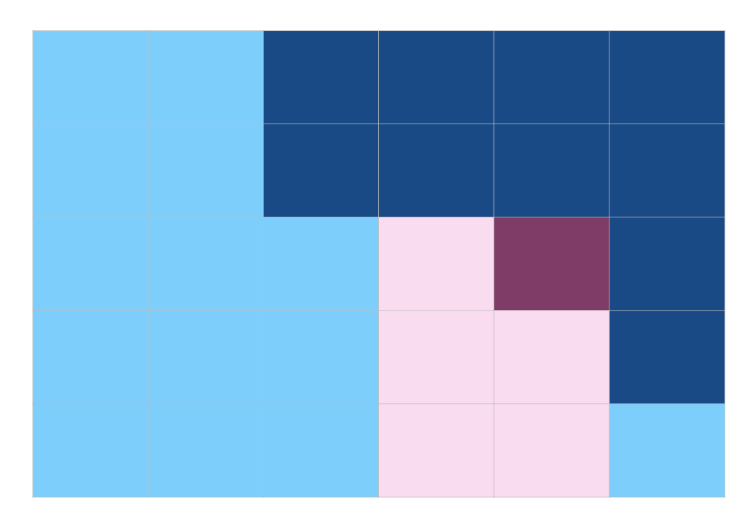
De Chaisemartin and d’Haultfoeuille (2020) and De Chaisemartin and d’Haultfoeuille (2024) introduce a method for multi-group, multi-period designs that accommodate a potentially non-binary treatment, which can change (increase or decrease) multiple times. For details, see Chaisemartin et al. (2024). Here, we demonstrate only the basic usage for a binary, staggered treatment.
When calling did_multiplegt_dyn, specify the outcome, treatment, unit index (group), and time index (time). The effects option determines how many event-study coefficients to estimate. For each period \(l\), the event-study effect represents the average change in the outcome for all switchers after receiving the treatment for \(l\) periods, compared to remaining at their initial treatment level. The placebo option specifies how many placebo coefficients to compute. For each placebo period \(k\), the command compares the outcome evolution of switchers and their controls \(k\) periods before the switchers’ first treatment change.
See a simple illustration below with \(l = 2\) (number of lags, capturing post-treatment effects) and \(k = 2\) (number of leads, capturing pre-treatment placebo effects).
In the following example, we set \(l = 12\) and \(k = 9\).
didm.results <- did_multiplegt_dyn(
      df = df.use,
      outcome = "nat_rate_ord",
      group = "bfs",
      controls = NULL,
      time = "year",
      treatment = "indirect",
      effects = 12,
      placebo = 9,
      cluster = "bfs",
      graph_off = TRUE
    )
print(didm.results)
#>
#> ----------------------------------------------------------------------
#>        Estimation of treatment effects: Event-study effects
#> ----------------------------------------------------------------------
#>              Estimate SE      LB CI    UB CI   N      Switchers
#> Effect_1     0.57568  0.38326 -0.17550 1.32686 11,978 514
#> Effect_2     1.53469  0.37166 0.80626  2.26313 11,000 425
#> Effect_3     1.58178  0.51351 0.57533  2.58823 10,051 357
#> Effect_4     0.88318  0.43757 0.02555  1.74081 9,183  352
#> Effect_5     0.36472  0.56355 -0.73981 1.46925 8,114  164
#> Effect_6     2.10445  0.79225 0.55167  3.65724 7,225  143
#> Effect_7     2.60910  0.87922 0.88586  4.33234 6,336  116
#> Effect_8     2.48694  0.81815 0.88340  4.09048 5,500  97
#> Effect_9     2.58597  0.86840 0.88394  4.28801 4,674  80
#> Effect_10    2.10762  0.99419 0.15904  4.05620 4,030  63
#> Effect_11    1.53529  0.98735 -0.39989 3.47046 3,385  50
#> Effect_12    0.07510  0.54641 -0.99585 1.14605 2,813  46
#>
#> Test of joint nullity of the effects : p-value = 0.0003
#> ----------------------------------------------------------------------
#>     Average cumulative (total) effect per treatment unit
#> ----------------------------------------------------------------------
#>  Estimate        SE     LB CI     UB CI         N Switchers
#>   1.30795   0.30296   0.71416   1.90174    16,616     2,407
#> Average number of time periods over which a treatment effect is accumulated: 3.9722
#>
#> ----------------------------------------------------------------------
#>      Testing the parallel trends and no anticipation assumptions
#> ----------------------------------------------------------------------
#>              Estimate SE      LB CI    UB CI    N      Switchers
#> Placebo_1    -0.09058 0.33955 -0.75610 0.57493  11,052 512
#> Placebo_2    -0.13816 0.35653 -0.83693 0.56062  9,159  419
#> Placebo_3    0.75490  0.44430 -0.11592 1.62571  7,295  346
#> Placebo_4    -0.15443 0.39019 -0.91918 0.61032  6,427  341
#> Placebo_5    -1.20890 0.41806 -2.02828 -0.38952 5,393  153
#> Placebo_6    -0.93342 0.50462 -1.92246 0.05561  4,543  132
#> Placebo_7    -1.32200 0.68078 -2.65631 0.01231  2,888  70
#> Placebo_8    0.04786  0.63937 -1.20529 1.30100  1,529  47
#> Placebo_9    0.82479  1.00818 -1.15120 2.80078  429    17
#>
#> Test of joint nullity of the placebos : p-value = 0.0225
#>
#>
#> The development of this package was funded by the European Union.
#> ERC REALLYCREDIBLE - GA N. 101043899
Again, we make an event study plot using esplot.
T.post <- dim(didm.results$results$Effects)[1]
T.pre <- dim(didm.results$results$Placebos)[1]
didm.vis <- rbind(didm.results$results$Placebos,didm.results$results$Effects)
didm.vis <- as.data.frame(didm.vis)
didm.vis[,'Time'] <- c(c(-1:-(T.pre)),c(1:T.post))
est.dynamic <- didm.vis[,c(9,1,2,3,4)]
colnames(est.dynamic) <- c("T","estimate","se","lb","ub")
p.didm <- esplot(est.dynamic,Period = 'T',Estimate = 'estimate',
                               SE = 'se', xlim = c(-9, 9))
p.didm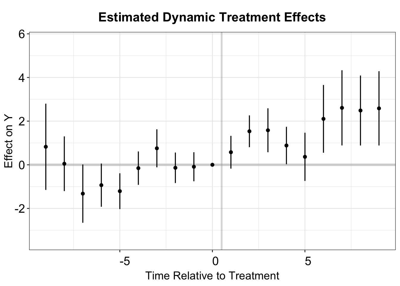
5.2.9 PanelMatch
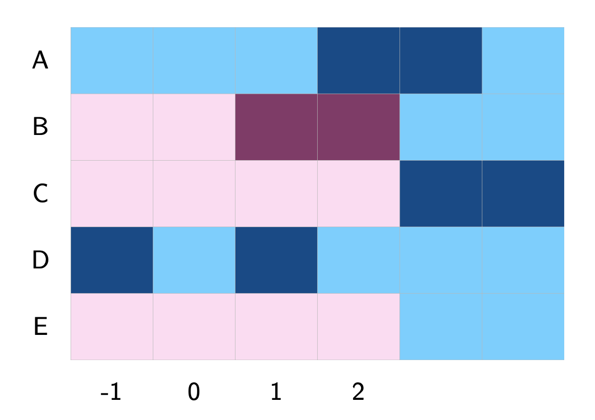
Imai, Kim, and Wang (2023) propose a matching method, similar in spirit to DIDm, for panel data analysis. It allows researchers to match each treated observation for a given unit in a particular period with untreated observations from other units in the same period that have similar treatment, outcome, or covariate histories. Their package is called PanelMatch.
The PanelMatch function in PanelMatch creates matched sets. The option lag = 3 specifies that pre-treatment history should span three periods, while lead = c(0:3) sets the lead window to include four post-treatment periods. Note that the terms lead and lag here are opposite to their traditional usage in a dynamic TWFE specification, where lags correspond to post-treatment effects and leads correspond to pre-treatment placebo effects.
To assign equal weights to all control units in each matched set, we set refinement.method = "none" (without matching on controls). Notably, by matching on treatment history and defining the lead window, PanelMatch uses only the subset of treated units with three pre-treatment periods and four post-treatment periods to compute the average treatment effects.
The PanelMatch estimator is equivalent to the DIDmulitple estimator proposed by Chaisemartin and D’Haultfœuille (2020) if we only match on the last pre-treatment period and only estimate the treatment effect at the first post-treatment period.
df.pm <- df.use
# we need to convert the unit and time indicator to integer
df.pm[,"bfs"] <- as.integer(as.factor(df.pm[,"bfs"]))
df.pm[,"year"] <- as.integer(as.factor(df.pm[,"year"]))
df.pm <- df.pm[,c("bfs","year","nat_rate_ord","indirect")]

# Pre-processes and balances panel data
df.pm <- PanelData(panel.data = df.pm,
                    unit.id = "bfs",
                    time.id = "year",
                    treatment = "indirect",
                    outcome = "nat_rate_ord")

PM.results <- PanelMatch(lag=3,
                         refinement.method = "none",
                         panel.data = df.pm,
                         qoi = "att",
                         lead = c(0:3),
                         match.missing = TRUE)

## For pre-treatment dynamic effects
PM.results.placebo <- PanelMatch(lag=3,
                         refinement.method = "none",
                         panel.data = df.pm,
                         qoi = "att",
                         lead = c(0:3),
                         match.missing = TRUE,
                         placebo.test = TRUE)
We can estimate the ATT and dynamic treatment effects using the function PanelEstimate. To obtain the ATT, we set the option pooled = TRUE. The standard error is calculated using a block bootstrapping method. This is different from the standard boostrapping method, which is not valid for matching estimators .
# ATT
PE.results.pool <- PanelEstimate(PM.results, panel.data = df.pm, pooled = TRUE)
summary(PE.results.pool)
#>      estimate std.error      2.5%    97.5%
#> [1,] 1.177674 0.3612923 0.4763911 1.891943
We can also use the function PanelEstimate to estimate the dynamic treatment effects at post-treatment periods. Additionally, for pre-treatment periods, PanelMatch offers the function placebo_test to compute the change in outcomes for each pre-treatment period in the lag window compared to the last pre-treatment period.
# Dynamic Treatment Effects
PE.results <- PanelEstimate(PM.results, panel.data = df.pm)
PE.results.placebo <- placebo_test(PM.results.placebo, panel.data = df.pm, plot = F)

# obtain lead and lag (placebo) estimates
est_lead <- as.vector(PE.results$estimate)
est_lag <- as.vector(PE.results.placebo$estimates)
sd_lead <- apply(PE.results$bootstrapped.estimates,2,sd)
sd_lag <- apply(PE.results.placebo$bootstrapped.estimates,2,sd)
coef <- c(est_lag, 0, est_lead)
sd <- c(sd_lag, 0, sd_lead)
pm.output <- cbind.data.frame(ATT=coef, se=sd, t=c(-2:4))

# plot
p.pm <- esplot(data = pm.output,Period = 't',
               Estimate = 'ATT',SE = 'se')
p.pm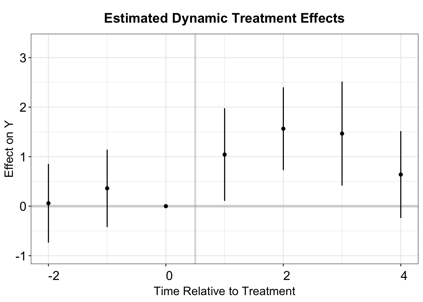
5.2.10 Imputation Method
Now, we return to the imputation method, which fect is originally designed to implement. See a simple illustration below. For details, see Chapter 2.
For a fair comparison, we implement this estimator—the fixed effects counterfactual (fect) estimator—based on a TWFE model. The estimated ATT is 1.506, with a standard error of 0.197.
The fect function stores the estimated dynamic treatment effects obtained using the counterfactual method in the object est.att. Uncertainty estimates are derived through a nonparametric clustered bootstrap/jackknife procedure.
fect.output <- as.matrix(out.fect$est.att)
head(fect.output)
#>             ATT      S.E.    CI.lower  CI.upper   p.value count
#> -17 -0.01985591 0.4765042 -0.95378688 0.9140751 0.9667618    89
#> -16  0.07269638 0.2331293 -0.38422873 0.5296215 0.7551708   157
#> -15 -0.21365489 0.2530582 -0.70963976 0.2823300 0.3985065   162
#> -14 -0.13153052 0.1606427 -0.44638437 0.1833233 0.4129137   350
#> -13  0.46902947 0.2010303  0.07501736 0.8630416 0.0196414   371
#> -12  0.24357664 0.1995137 -0.14746305 0.6346163 0.2221422   398
Borusyak, Jaravel, and Spiess (2024) also provide the didimputation package to estimate the ATT using the same approach as Liu, Wang, and Xu (2024).
df.impute <- df.use
df.impute[which(is.na(df.impute$FirstTreat)),"FirstTreat"] <- 0
# above, replace NA with 0

out.impute <- did_imputation(data = df.impute,
                               yname = "nat_rate_ord",
                               gname = "FirstTreat",
                               tname = "year",
                               idname = "bfs",
                               cluster_var = "bfs")
out.impute
#> # A tibble: 1 × 6
#>   lhs          term  estimate std.error conf.low conf.high
#>   <chr>        <chr>    <dbl>     <dbl>    <dbl>     <dbl>
#> 1 nat_rate_ord treat     1.51     0.187     1.14      1.87
We can use esplot() to create the event study plot as before. Additionally, the fect package offers more advanced visualization tools specifically designed for imputation estimators (see the previous chapters and the next chapter).
fect.output <- as.data.frame(fect.output)
fect.output$Time <- c(-17:18)
p.fect <- esplot(fect.output,Period = 'Time',Estimate = 'ATT',
                   SE = 'S.E.',CI.lower = "CI.lower",
                   CI.upper = 'CI.upper',xlim = c(-12,10))
p.fect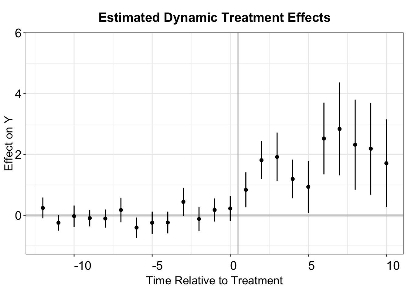
The didimputation package also supports event study estimation, producing numerically equivalent estimates for dynamic treatment effects in the post-treatment period. However, didimputation uses a distinct TWFE regression applied only to untreated observations to obtain pre-treatment estimates and test for parallel trends. In this case, we specify pretrends = c(-13:-1) to compute regression coefficients for pre-treatment periods ranging from -13 to -1.
model.impute <- did_imputation(data = df.impute,
                               yname = "nat_rate_ord",
                               gname = "FirstTreat",
                               tname = "year",
                               idname = "bfs",
                               cluster_var = "bfs",
                               pretrends = c(-13:-1),
                               horizon = TRUE)
model.impute$term <- as.numeric(model.impute$term)+1
# above, set 1 as the first post-treatment period

# plot
to_plot <- as.data.frame(model.impute)
esplot(data=to_plot,Period = "term",
       Estimate = 'estimate', SE = 'std.error',
       xlim = c(-12,10))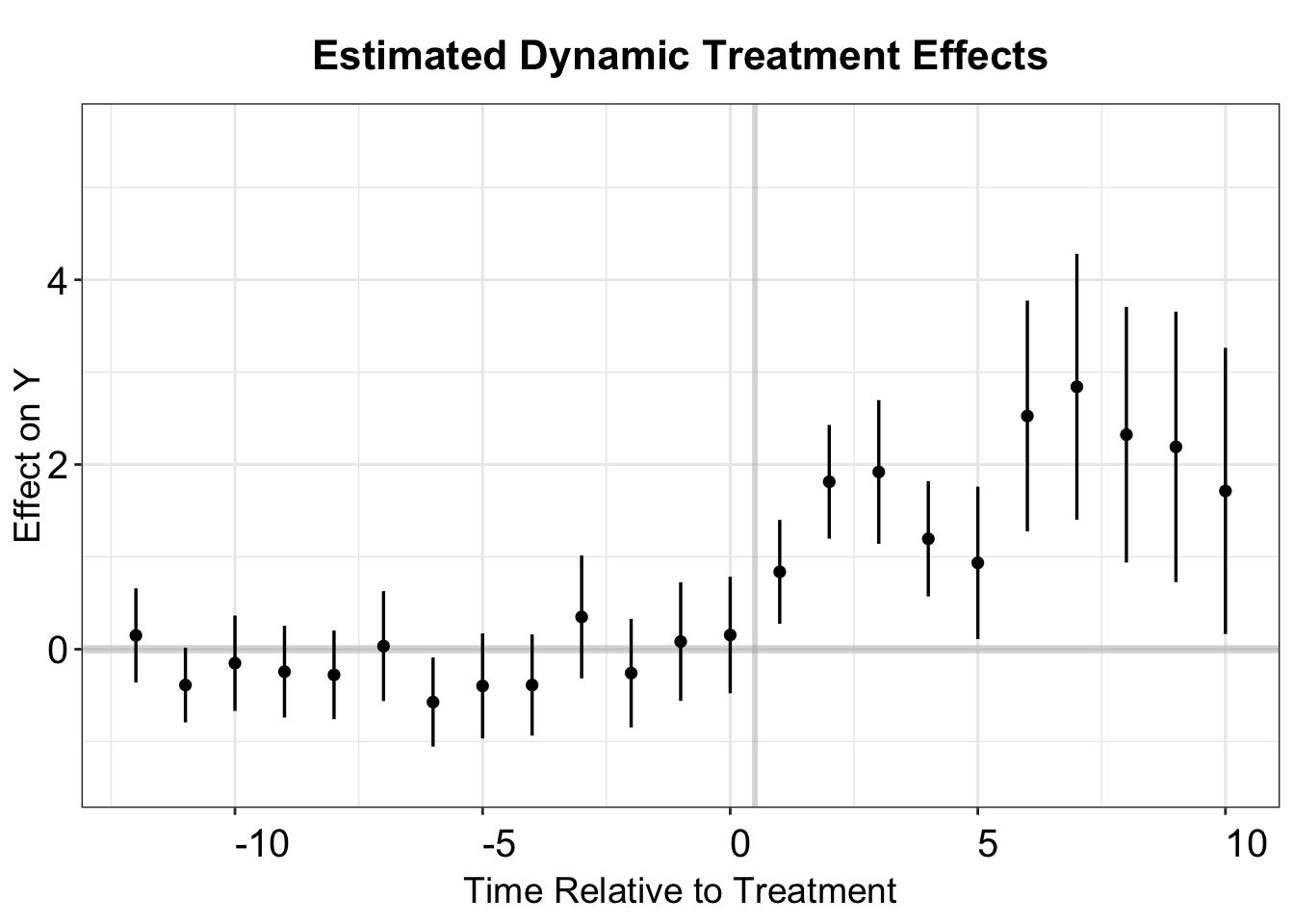
out.impute
#> # A tibble: 1 × 6
#>   lhs          term  estimate std.error conf.low conf.high
#>   <chr>        <chr>    <dbl>     <dbl>    <dbl>     <dbl>
#> 1 nat_rate_ord treat     1.51     0.187     1.14      1.87
To compare the results with those obtained using the PanelMatch method, fect provides the option to compute the ATT for the subset of units with three pre-treatment periods and four post-treatment periods. This can be done by setting balance.period = c(-2,4), which includes periods -2, -1, and 0 for pre-treatment and 1, 2, 3, and 4 for post-treatment.
out.fect.balance <- fect(nat_rate_ord~indirect, data = df,
                         index = c("bfs","year"),
                         method = 'fe', se = TRUE,
                         balance.period = c(-2,4))
# att
print(out.fect.balance$est.balance.avg)
#>       ATT.avg      S.E. CI.lower CI.upper      p.value
#> [1,] 1.711554 0.2279724 1.264736 2.158372 6.017409e-14

# event study plot
fect.balance.output <- as.data.frame(out.fect.balance$est.balance.att)
fect.balance.output$Time <- c(-2:4)
p.fect.balance <- esplot(fect.balance.output,Period = 'Time',
                         Estimate = 'ATT', SE = 'S.E.',
                         CI.lower = "CI.lower",
                         CI.upper = 'CI.upper')
p.fect.balance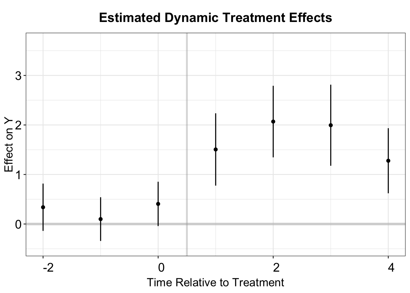
5.3 With Treatment Reversals
We use data from Grumbach and Sahn (2020) to demonstrate methods that can accommodate treatment reversals, where treatment can switch on and off. These methods include TWFE, PanelMatch, and the imputation estimator.
In the original paper, the authors use district by election-cycle panel data from U.S. House general elections between 1980 and 2012, arguing that the presence of Asian (Black/Latino) candidates in general elections increases the proportion of campaign contributions from Asian (Black/Latino) donors. Here, we focus specifically on the effects of Asian candidates, as shown in the top left panel of Figure 5 in the paper.
data(fect)
data <- gs2020
data$cycle <- as.integer(as.numeric(data$cycle/2))
head(data)
#> # A tibble: 6 × 9
#>   cycle district_final general_sharetotal_A_all general_sharetotal_B_all
#>   <int> <chr>                             <dbl>                    <dbl>
#> 1   991 AK1                             0                         0
#> 2   992 AK1                             0                         0.0506
#> 3   993 AK1                             0.0362                    0.0723
#> 4   994 AK1                             0.0157                    0.0104
#> 5   995 AK1                             0                         0.0188
#> 6   996 AK1                             0.00651                   0.0332
#> # ℹ 5 more variables: general_sharetotal_H_all <dbl>, cand_A_all <dbl>,
#> #   cand_B_all <dbl>, cand_H_all <dbl>, dfe <dbl>
5.3.1 Visualizing Data
In our analysis, district_final and cycle serve as the unit and time indices, respectively. The treatment variable, cand_A_all, indicates the presence of an Asian candidate, while the outcome variable, general_sharetotal_A_all, represents the proportion of donations from Asian donors. The covariates included are cand_H_all, indicating a Hispanic candidate, and cand_B_all, indicating a Black candidate.
As usual, we use the panelView package to examine treatment conditions and missing values in the data. We set by.timing = TRUE to organize units by treatment timing. Below, we can see that this dataset has missing values in the outcome variable, and the treatment may switch on and off.
y <- "general_sharetotal_A_all"
d <- "cand_A_all"
unit <- "district_final"
time <- "cycle"
controls <- c("cand_H_all", "cand_B_all")
index <- c("district_final", "cycle")

panelview(Y=y, D=d, X=controls, index = index, data = data,
          xlab = "Time Period", ylab = "Unit", gridOff = TRUE,
          by.timing = TRUE, cex.legend=5, cex.axis= 5,
          cex.main = 10, cex.lab = 5)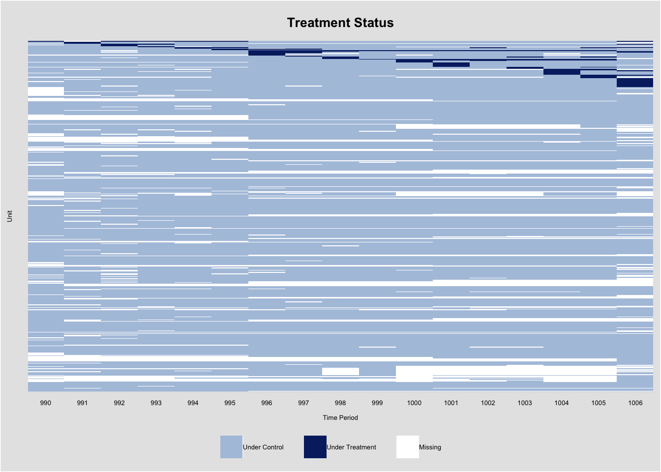
5.3.2 TWFE
First, we estimate the effect of an Asian candidate on the proportion of Asian donations using the TWFE estimator. The estimated coefficient is 0.128, with a standard error of 0.025, clustered at the district level.
model.twfe <- feols(general_sharetotal_A_all ~ cand_A_all +
                      cand_H_all + cand_B_all | district_final + cycle,
                    data=data, cluster = "district_final")
summary(model.twfe)
#> OLS estimation, Dep. Var.: general_sharetotal_A_all
#> Observations: 6,847
#> Fixed-effects: district_final: 489,  cycle: 17
#> Standard-errors: Clustered (district_final)
#>            Estimate Std. Error t value   Pr(>|t|)
#> cand_A_all 0.128098   0.025007 5.12256 4.3480e-07 ***
#> cand_H_all 0.012181   0.005274 2.30980 2.1316e-02 *
#> cand_B_all 0.010456   0.004594 2.27615 2.3269e-02 *
#> ---
#> Signif. codes:  0 '***' 0.001 '**' 0.01 '*' 0.05 '.' 0.1 ' ' 1
#> RMSE: 0.049535     Adj. R2: 0.275898
#>                  Within R2: 0.083964
To estimate dynamic treatment effects using TWFE, we first use the get.cohort function to determine the relative period to treatment. Next, we generate the treated unit indicator treat using the following steps:
- Set
treat = 0for observations of units that have never been treated.
- For treated units, if the treatment switches on and off, assign
treat = 1only for observations before the last treatment exit. For example, if a unit’s treatment status sequence is0, 0, 0, 1, 1, 0, 0, we settreat = 1only for the first five observations. This approach assumes no carryover effects, meaning treatment affects only the current period.
- Finally, we interact the dummy variable
treatwith the relative period index in a two-way fixed effects regression to estimate dynamic treatment effects.
data_cohort <- get.cohort(data, index = index, D=d,start0 = TRUE)
# Generate a dummy variable treat
data_cohort$treat <- 0
data_cohort[which(data_cohort$Cohort!='Control'),'treat'] <- 1
data_cohort[which(is.na(data_cohort$Time_to_Treatment)), "treat"] <- 0

# remove observations that starts with treated status
remove <- intersect(which(is.na(data_cohort$Time_to_Treatment)),
                    which(data_cohort[,d]==1))
if(length(remove)>0){data_cohort <- data_cohort[-remove,]}

# replace missingness in Time_to_Treatment with an arbitrary number
data_cohort[which(is.na(data_cohort$Time_to_Treatment)), "Time_to_Treatment"] <- 999

twfe.est <- feols(general_sharetotal_A_all ~
                    i(Time_to_Treatment, treat, ref = -1) +
                    cand_H_all +cand_B_all | district_final + cycle,
                  data = data_cohort, cluster = "district_final")
We then visualize the estimated dynamic treatment.
5.3.3 PanelMatch
PanelMatch can handle treatment reversals but uses only a subset of the data based on the specified numbers of leads and lags. DIDmultiple, proposed by Chaisemartin and D’Haultfœuille (2020), can also accommodate treatment reversals. However, its current implementation in R, DIDmultiplegtDYN, focuses only on the first switch from the control condition to the treatment condition for each unit. Therefore, we use PanelMatch to illustrate how matching methods work in this more general setting.
In this case, we use a subset of treated units with four pre-treatment periods and one post-treatment period to estimate the average treatment effects.
df.pm <- data_cohort
# we need to convert the unit and time indicator to integer
df.pm[,"district_final"] <- as.integer(as.factor(df.pm[,"district_final"]))
df.pm[,"cycle"] <- as.integer(as.factor(df.pm[,"cycle"]))
df.pm <- df.pm[,c("district_final","cycle","cand_A_all",
                  "general_sharetotal_A_all")]

# Pre-processes and balances panel data
df.pm <- PanelData(panel.data = df.pm,
                    unit.id = "district_final",
                    time.id = "cycle",
                    treatment = "cand_A_all",
                    outcome = "general_sharetotal_A_all")

PM.results <- PanelMatch(lag=4,
                         refinement.method = "none",
                         panel.data = df.pm,
                         qoi = "att",
                         lead = 0,
                         match.missing = TRUE)

## For pre-treatment dynamic effects
PM.results.placebo <- PanelMatch(lag=4,
                         refinement.method = "none",
                         panel.data = df.pm,
                         qoi = "att",
                         lead = 0,
                         match.missing = TRUE,
                         placebo.test = TRUE)
The ATT estimate is 0.124, with a standard error of 0.023.
PE.results.pool <- PanelEstimate(PM.results, panel.data = df.pm, pooled = TRUE)
summary(PE.results.pool)
#>      estimate  std.error       2.5%     97.5%
#> [1,] 0.124243 0.02311266 0.08060554 0.1712501
We obtain the dynamic treatment effects using the same approach as demonstrated in the case of Hainmueller and Hangartner (2019) with the esplot function.
# Dynamic Treatment Effects
PE.results <- PanelEstimate(PM.results, panel.data = df.pm)
PE.results.placebo <- placebo_test(PM.results.placebo, panel.data = df.pm,
                                   plot = FALSE)

est_lead <- as.vector(PE.results$estimate)
est_lag <- as.vector(PE.results.placebo$estimates)
sd_lead <- apply(PE.results$bootstrapped.estimates,2,sd)
sd_lag <- apply(PE.results.placebo$bootstrapped.estimates,2,sd)
coef <- c(est_lag, 0, est_lead)
sd <- c(sd_lag, 0, sd_lead)
pm.output <- cbind.data.frame(ATT=coef, se=sd, t=c(-3:1))

# plot
p.pm <- esplot(data = pm.output,Period = 't',
               Estimate = 'ATT',SE = 'se')
p.pm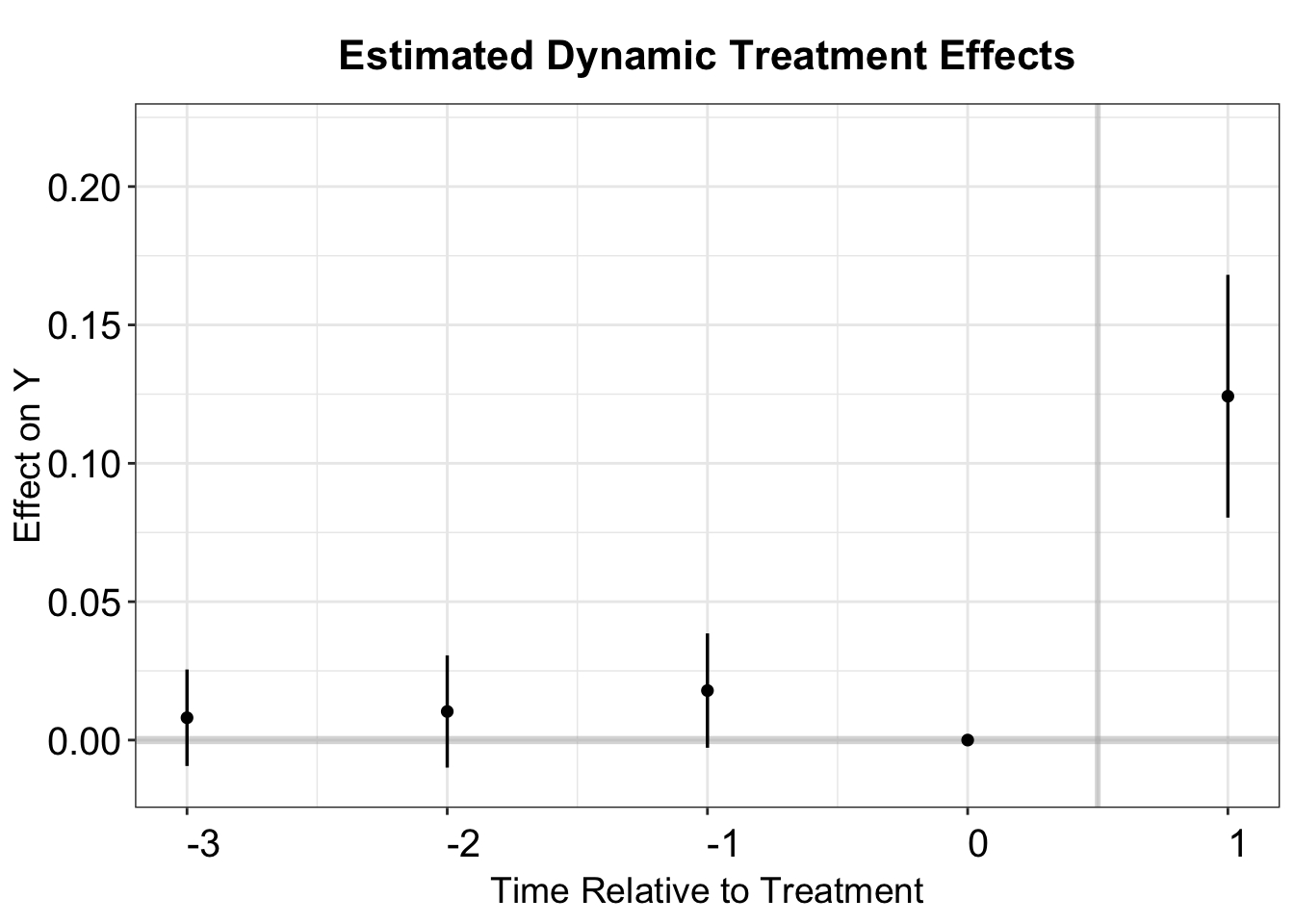
5.3.4 Imputation Method
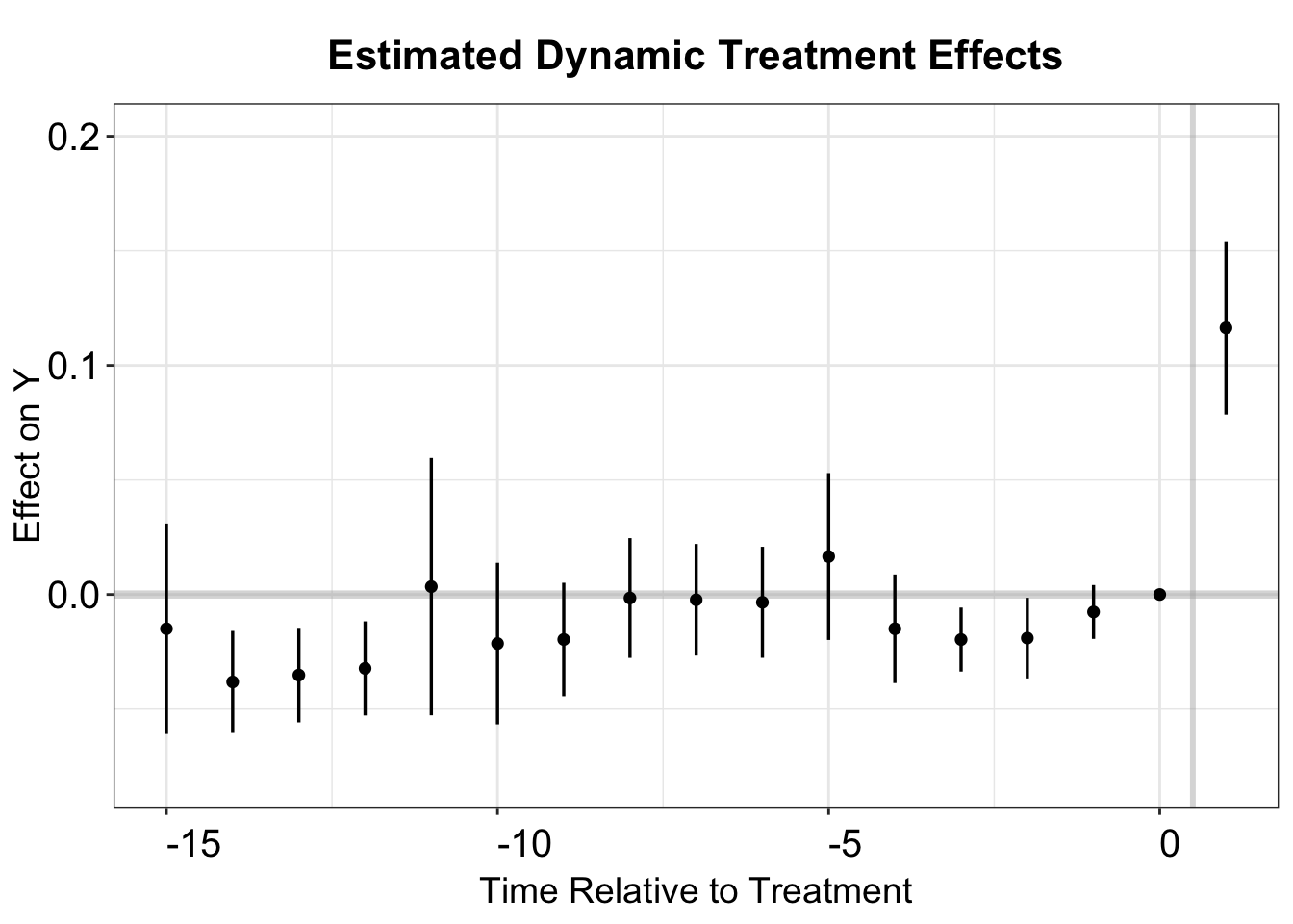
Now we return to the imputation method proposed by Borusyak, Jaravel, and Spiess (2024) and Liu, Wang, and Xu (2024). The estimated ATT is 0.127, with a standard error of 0.025. Both are very close to the TWFE estimates.
model.fect <- fect(Y = "general_sharetotal_A_all", D = "cand_A_all",
                   X= c("cand_H_all", "cand_B_all"), data = data,
                   method = "fe", index = index, se = TRUE,
                   parallel = TRUE, seed = 1234, force = "two-way")

print(model.fect$est.avg)
#>        ATT.avg       S.E.   CI.lower CI.upper      p.value
#> [1,] 0.1277491 0.02469477 0.07934829  0.17615 2.302096e-07
We visualize the estimated dynamic treatment for the counterfactual estimator in the same way.
fect.output <- as.data.frame(model.fect$est.att)
fect.output$Time <- c(-15:10)
p.fect <- esplot(fect.output,Period = 'Time',Estimate = 'ATT',
                   SE = 'S.E.',CI.lower = "CI.lower",
                   CI.upper = 'CI.upper', xlim = c(-15,1))
p.fect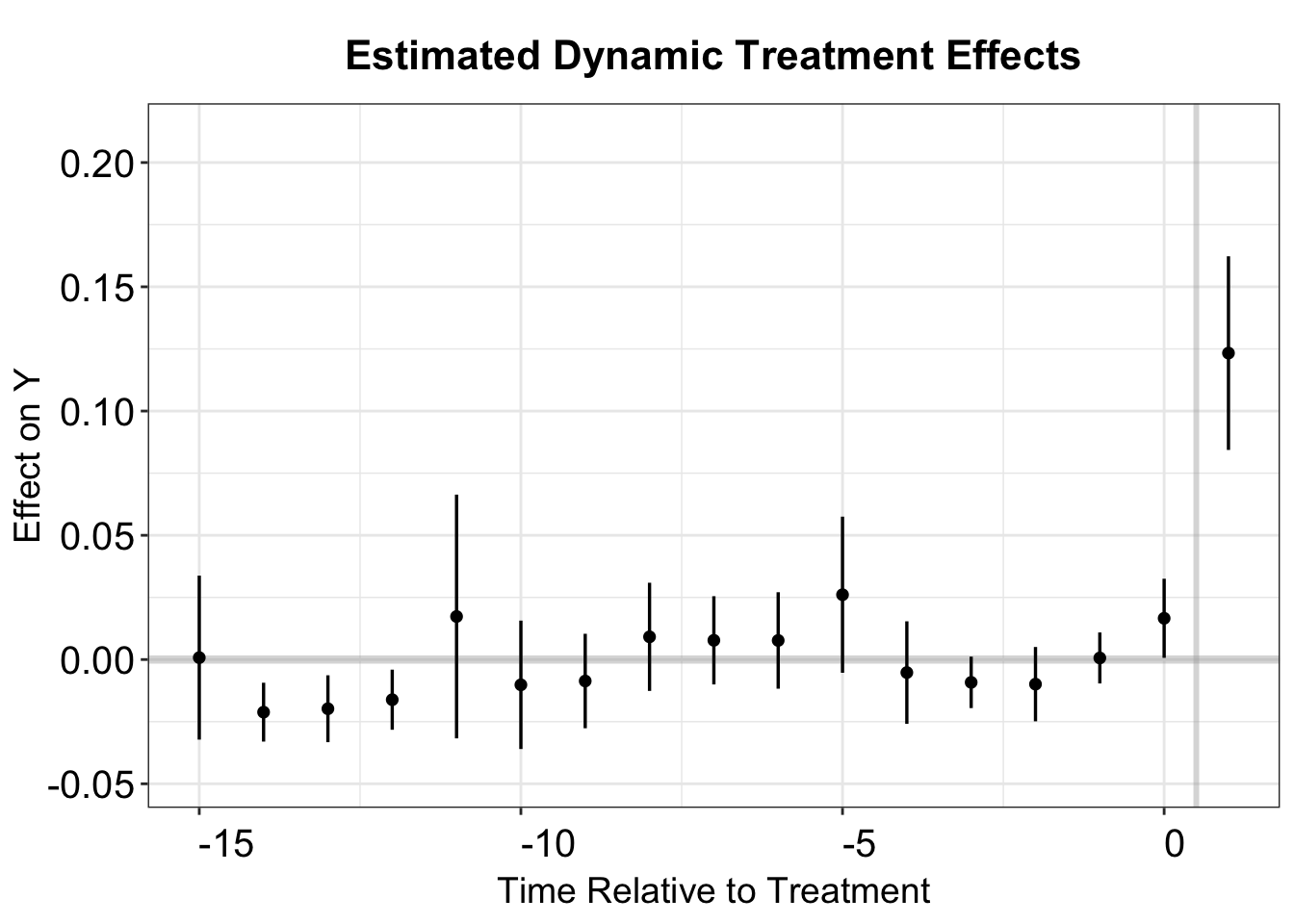
The plot function shipped with fect can make the event study plot easily with a bar plot in the bottom indicating the number of treated units for each period.
plot(model.fect)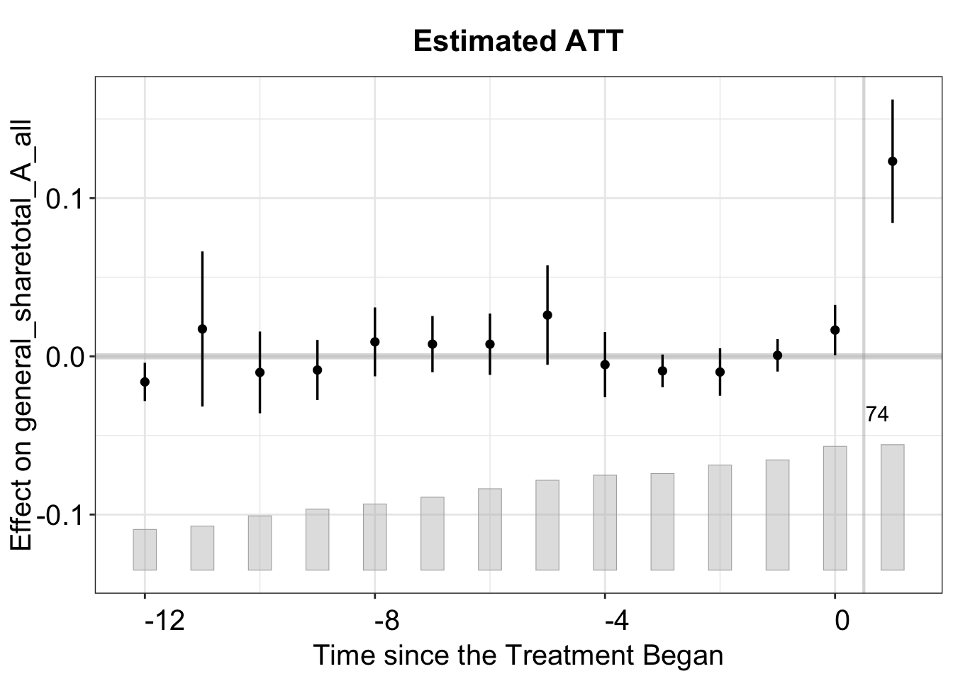
We can visualize the period-wise ATT relative to the exit of the treatment by setting type = "exit".
plot(model.fect, type = 'exit')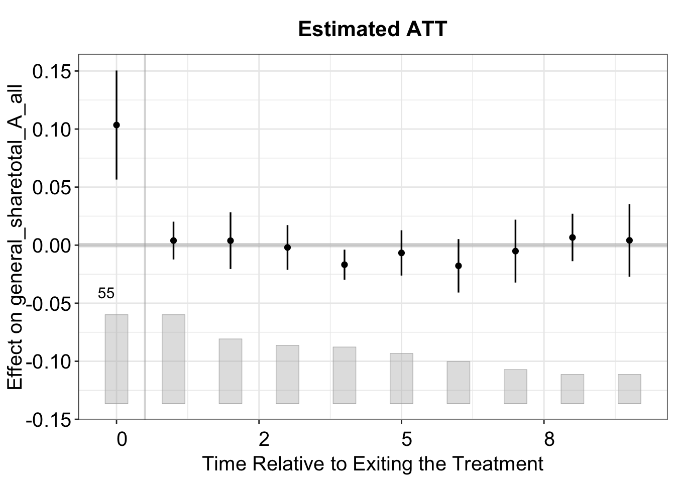
As discussed in Chapter 2, fect provides various diagnostic tests, including the \(F\) test, placebo test, equivalence tests, and test for no-carryover effects. The figure below presents the results of a placebo test, where we set placebo.period = c(-2, 0), specifying that the placebo periods include the three periods preceding treatment onset.
out.fect.p <- fect(Y = y, X = controls, D = d, data = data, index = index,
                   method = 'fe', se = TRUE, placeboTest = TRUE,
                   placebo.period = c(-2,0))

plot(out.fect.p, proportion = 0.1, stats = "placebo.p")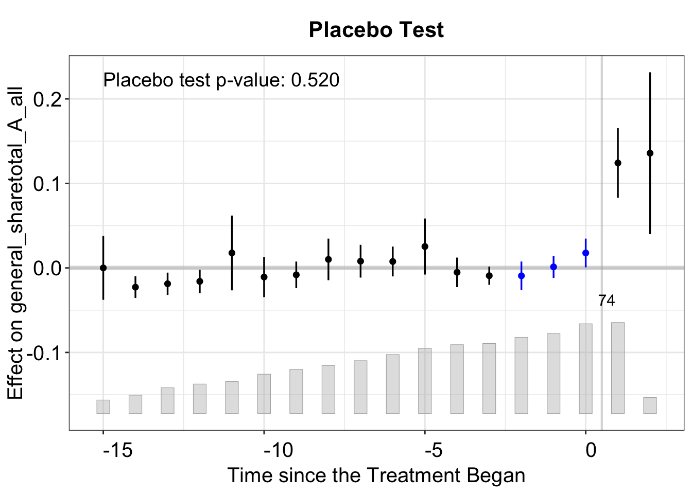
We then test for carryover effects by setting carryoverTest = TRUE and carryover.period = c(1,2), which removes observations from periods after treatment has ended from the data used to fit the model. The test then assesses whether the estimated ATT in this range is significantly different from zero.
out.fect.c <- fect(Y = y, X = controls, D = d, data = data, index = index,
                   method = 'fe', se = TRUE, carryoverTest = TRUE, carryover.period = c(1,2))

# plot
plot(out.fect.c,  stats = "carryover.p", ylim = c(-0.15, 0.20))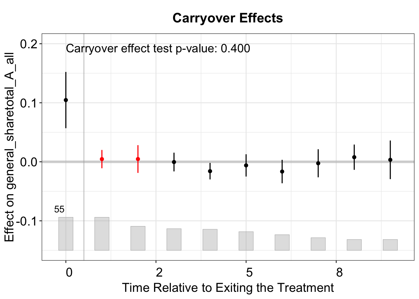
To compare with the estimates from PanelMatch, we can construct a balanced sample by setting balance.period = c(-3,1)), ensuring that both methods use the same set of treated observations. The ATT estimate is similar but slightly larger than that obtained using the full sample.
out.fect.balance <- fect(Y = y, X = controls, D = d, data = data,
                         index = index, method = 'fe', se = TRUE,
                         balance.period = c(-3,1))

# att
print(out.fect.balance$est.balance.avg)
#>        ATT.avg       S.E.   CI.lower  CI.upper      p.value
#> [1,] 0.1399293 0.02657371 0.08784574 0.1920128 1.396545e-07

# event study plot
fect.balance.output <- as.data.frame(out.fect.balance$est.balance.att)
fect.balance.output$Time <- c(-3:1)
p.fect.balance <- esplot(fect.balance.output,Period = 'Time',Estimate = 'ATT',
                   SE = 'S.E.',CI.lower = "CI.lower",
                   CI.upper = 'CI.upper')
p.fect.balance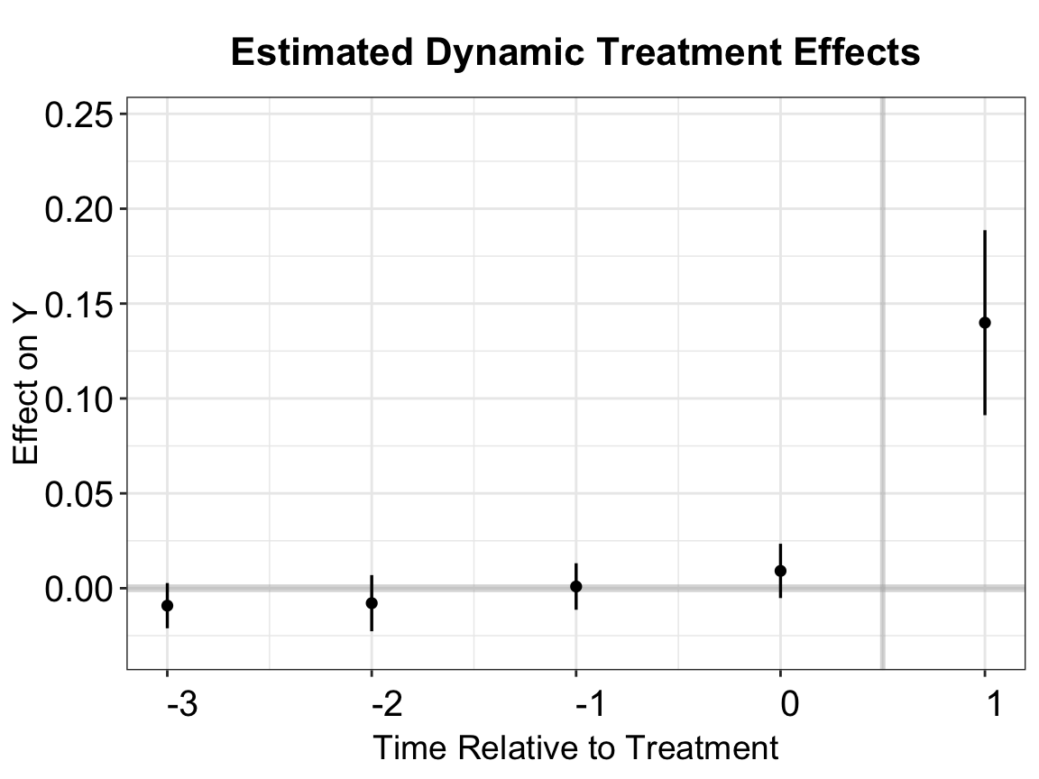
5.4 did_wrapper()
While the preceding sections have meticulously detailed the individual implementation of various HTE-robust DID estimators, the fect package also provides a convenient function, did_wrapper, that can significantly streamline this process for several common methods.
The did_wrapper function can execute methods such as:
Two-Way Fixed Effects (TWFE): by setting
method = "twfe". This replicates the dynamic TWFE event study estimation.Stacked DID: by setting
method = "st". This implements the stacked difference-in-differences approach by Cengiz et al. (2019).Interaction Weighted (IW) DID: by setting
method = "iw". This corresponds to the Sun and Abraham (2021) estimator.-
Callaway and Sant’Anna (CSDID):
- Using never-treated controls:
method = "cs_never". - Using not-yet-treated controls:
method = "cs_notyet".
- Using never-treated controls:
DIDmultiplegtDYN (“didm”): by setting
method = "didm". This calls the estimator by Chaisemartin and D’Haultfœuille (2020).
You could use did_wrapper to implement Stacked DID as follows:
res_st <- did_wrapper(
  data   = hh2019,
  Y      = "nat_rate_ord",
  D      = "indirect",
  index  = c("bfs", "year"),
  method = "st",
  se     = "default"
)
print(res_st)
#> $est.avg
#>    ATT.avg      S.E. CI.lower CI.upper p.value
#> 1 1.668611 0.1823702 1.311166 2.026057       0
#>
#> $est.att
#>             ATT      S.E.    CI.lower    CI.upper      p.value count
#> -17 -0.32876531 0.6246666 -1.55311188  0.89558126 5.986761e-01    89
#> -16 -0.08402861 0.3726755 -0.81447262  0.64641541 8.216106e-01   157
#> -15 -0.23704732 0.3890202 -0.99952696  0.52543232 5.422961e-01   162
#> -14 -0.33039222 0.3358986 -0.98875356  0.32796912 3.253088e-01   350
#> -13  0.21942491 0.3595513 -0.48529567  0.92414549 5.416802e-01   371
#> -12 -0.13145445 0.3443222 -0.80632599  0.54341709 7.026265e-01   398
#> -11 -0.58822817 0.3113593 -1.19849231  0.02203597 5.886148e-02   417
#> -10 -0.26344604 0.3437730 -0.93724111  0.41034903 4.434757e-01   434
#> -9  -0.54375457 0.3218685 -1.17461692  0.08710778 9.114884e-02   451
#> -8  -0.56120024 0.3065223 -1.16198397  0.03958348 6.712105e-02   464
#> -7  -0.09265692 0.3389478 -0.75699462  0.57168077 7.845716e-01   468
#> -6  -0.58880594 0.3070364 -1.19059721  0.01298533 5.514811e-02   503
#> -5  -0.47516514 0.3257192 -1.11357485  0.16324457 1.446152e-01   503
#> -4  -0.39993315 0.3112587 -1.01000020  0.21013391 1.988308e-01   503
#> -3   0.23387391 0.3587515 -0.46927899  0.93702681 5.144588e-01   503
#> -2  -0.24046110 0.3308839 -0.88899360  0.40807140 4.673954e-01   508
#> -1  -0.01674545 0.3466380 -0.69615598  0.66266509 9.614706e-01   512
#> 1    0.63988908 0.3639778 -0.07350735  1.35328550 7.873995e-02   514
#> 2    1.63436478 0.3698039  0.90954919  2.35918037 9.890902e-06   425
#> 3    1.78039699 0.4911171  0.81780741  2.74298657 2.887398e-04   357
#> 4    1.10329058 0.4123146  0.29515403  1.91142713 7.454073e-03   352
#> 5    0.85952703 0.4895732 -0.10003645  1.81909052 7.914546e-02   164
#> 6    2.44794424 0.7113218  1.05375357  3.84213491 5.787078e-04   143
#> 7    2.80029784 0.8125259  1.20774702  4.39284866 5.680868e-04   116
#> 8    2.29340055 0.7978800  0.72955573  3.85724536 4.048373e-03    97
#> 9    2.38558084 0.7977891  0.82191421  3.94924747 2.787584e-03    80
#> 10   2.20907842 0.8509387  0.54123858  3.87691827 9.430266e-03    63
#> 11   1.90401019 0.9458353  0.05017309  3.75784728 4.410976e-02    50
#> 12   0.51499900 0.5518266 -0.56658115  1.59657914 3.506845e-01    46
#> 13   3.95439028 2.2940011 -0.54185185  8.45063241 8.474465e-02    11
#> 14   4.39078917 2.3089816 -0.13481484  8.91639318 5.722179e-02    11
#> 15   4.61626419 3.4608264 -2.16695557 11.39948394 1.822491e-01    11
#> 16   1.18977420 1.3883525 -1.53139661  3.91094501 3.914623e-01    11
#> 17   6.75219353 4.8161984 -2.68755529 16.19194236 1.609225e-01     6
#> 18   5.95993087 2.7217298  0.62534037 11.29452137 2.854176e-02     2
#>
#> attr(,"class")
#> [1] "did_wrapper"
It also supports a bootstrap variance estimator via the se argument: se = "default" uses the standard errors from the underlying estimator, while se = "boot" applies bootstrapping.
res_st <- did_wrapper(
  data   = hh2019,
  Y      = "nat_rate_ord",
  D      = "indirect",
  index  = c("bfs", "year"),
  method = "st",
  se     = "boot"
)
print(res_st)
#> $est.avg
#>    ATT.avg      S.E. CI.lower CI.upper p.value
#> 1 1.668611 0.1534711 1.375633 1.971987       0
#>
#> $est.att
#>             ATT      S.E.    CI.lower    CI.upper p.value count
#> -17 -0.32876531 0.4810330 -1.12285490  0.57164714    0.58    89
#> -16 -0.08402861 0.3012874 -0.64797971  0.51525186    0.70   157
#> -15 -0.23704732 0.2953517 -0.76212626  0.35680559    0.29   162
#> -14 -0.33039222 0.2714152 -0.79272912  0.23358912    0.23   350
#> -13  0.21942491 0.2890344 -0.33178761  0.72459257    0.49   371
#> -12 -0.13145445 0.2665237 -0.63100684  0.41685128    0.59   398
#> -11 -0.58822817 0.2484023 -1.05736153 -0.07216216    0.01   417
#> -10 -0.26344604 0.2592624 -0.71865197  0.27105658    0.25   434
#> -9  -0.54375457 0.2386946 -0.96988820 -0.06374556    0.00   451
#> -8  -0.56120024 0.2354756 -1.02699163 -0.12619824    0.02   464
#> -7  -0.09265692 0.2543527 -0.53622937  0.39539961    0.72   468
#> -6  -0.58880594 0.2182008 -1.02868448 -0.09888941    0.00   503
#> -5  -0.47516514 0.2418846 -0.93922164 -0.02119348    0.05   503
#> -4  -0.39993315 0.2176024 -0.82168391  0.01053239    0.07   503
#> -3   0.23387391 0.2733380 -0.27123450  0.76127646    0.37   503
#> -2  -0.24046110 0.2365958 -0.66558144  0.23387373    0.23   508
#> -1  -0.01674545 0.2589173 -0.48906967  0.46840020    0.94   512
#> 1    0.63988908 0.2775716  0.10053601  1.16851807    0.03   514
#> 2    1.63436478 0.2566250  1.18875117  2.21851162    0.00   425
#> 3    1.78039699 0.3692277  1.07448499  2.49065619    0.00   357
#> 4    1.10329058 0.2943419  0.55784252  1.67289834    0.00   352
#> 5    0.85952703 0.3843362  0.06690499  1.59218975    0.02   164
#> 6    2.44794424 0.5332701  1.44540549  3.48552863    0.00   143
#> 7    2.80029784 0.6736518  1.57998555  4.05695376    0.00   116
#> 8    2.29340055 0.6139933  1.08607879  3.53592396    0.00    97
#> 9    2.38558084 0.5981798  1.22807795  3.57941881    0.00    80
#> 10   2.20907842 0.7023539  0.94397421  3.58960577    0.00    63
#> 11   1.90401019 0.7723164  0.67990632  3.52267287    0.01    50
#> 12   0.51499900 0.4211106 -0.32987055  1.31777468    0.19    46
#> 13   3.95439028 1.9501400 -0.04355279  7.63775268    0.04    11
#> 14   4.39078917 2.0253850  0.24143529  8.28551603    0.02    11
#> 15   4.61626419 3.1358601 -1.16090502 10.02382283    0.19    11
#> 16   1.18977420 1.1263054 -0.61311691  3.15391525    0.45    11
#> 17   6.75219353 4.5381055 -3.42999995 12.60741060    0.00     6
#> 18   5.95993087 2.8364291  1.56016157 10.22661683    0.00     2
#>
#> attr(,"class")
#> [1] "did_wrapper"
Finally, esplot can be used to visualize the results. The did_wrapper function returns a list of objects, including the estimated coefficients and standard errors, which can be used to create event study plots.

5.5 How to Cite
Please cite the authors of the original papers for their innovations. If you find this tutorial helpful, you can cite Chiu et al. (2025).