Tutorial
iv_tutorial.RmdThe ivDiag package is a toolkit created for researchers to conduct estimation, inference, sensitivity analysis, and visualization with instrumental variable (IV) designs. It provides R implementations of the guidelines proposed in Lal et al. (2023), enabling researchers to obtain reliable and robust estimates of their IV models.
The package includes a range of functions to compute various standard errors (SEs), multiple types of F-statistics, and weak-IV robust confidence intervals (CIs). These features ensure that researchers can accurately capture the uncertainty associated with their IV estimates and make valid statistical inferences.
The package also integrates the Anderson-Rubin (AR) test and adjusted t-ratio inference from Lee et al. (2022), enhancing the validity and reliability of the package’s statistical inference capabilities.
Moreover, ivDiag offers the Local-to-Zero (LTZ) estimator (Conley, Hansen, and Rossi 2012), which allows for more precise estimation of the causal effect of interest. Additionally, the package provides functions to plot coefficients of two-stage least squares (2SLS) and ordinary least squares (OLS) regressions, enabling researchers to visually compare the differences between these two estimators and various inferential methods.
The estimation routines in the omnibous function ivDiag
return a list that can be sliced and appended to additional rows in
tables produced by modelsummary,
fixest::etable, and stargazer, among other tools. This
makes it easy for researchers to integrate ivDiag estimates
into their existing workflows.
Note that ivDiag is applicable for the one-treatment case only, although there can be multiple instruments.
ivDiag ships three datasets for illustration
purposes: rueda, gsz and
gsz_south. rueda is based on Rueda (2017), while the other two are based on
Guiso, Sapienza, and Zingales (2016).
Estimation and Inference
We use Rueda (2017) to illustrate
ivDiag’s estimation and inference functionalities. The
author studies the persistence of vote buying in developing democracies
despite the use of secret ballots and argues that brokers condition
future payments on published electoral results to enforce these
transactions and that this is effective only when the results of small
voting groups are available.
The study examines the relationship between polling station size and vote buying using three different measures of the incidence of vote buying, two at the municipality level and one at the individual level. The paper also considers other factors such as poverty and lack of education as potential explanations for why vote buying persists despite secret ballots.
The size of the polling station, predicted by the rules limiting the number of voters per polling station, is used as an instrument of the actual polling place size. The institutional rule predicts sharp reductions in the size of the average polling station of a municipality every time the number of registered voters reaches a multiple of the maximum number of voters allowed to vote in a polling station. Such sharp reductions are used as a source of exogenous variation in polling place size to estimate the causal effect of this variable on vote buying.
| Summary | |
|---|---|
| Unit of analysis | city |
| Treatment | the actual polling place size |
| Instrument | the predicted size of the polling station |
| Outcome | citizens’ reports of electoral manipulation |
| Model | Table5(1) |
Visualizing the first stage
Y <- "e_vote_buying" # Y: outcome of interest
D <-"lm_pob_mesa" # D: endogenous treatment
Z <- "lz_pob_mesa_f" # Z: instrumental variable
controls <- c("lpopulation", "lpotencial") # covariates of control variables
cl <- "muni_code" # clusters
weights <- FE <- NULL # no weights or fixed effects

# first stage (raw)
par(mar = c(4, 4, 2, 2))
plot(rueda$lz_pob_mesa_f, rueda$lm_pob_mesa, col = "#777777", cex = 0.5,
     main = "Raw Data", xlab = "Instrument", ylab = "Treatment")
abline(lm(lm_pob_mesa ~ lz_pob_mesa_f, data = rueda),
       col = 2, lwd = 2, lty = 2)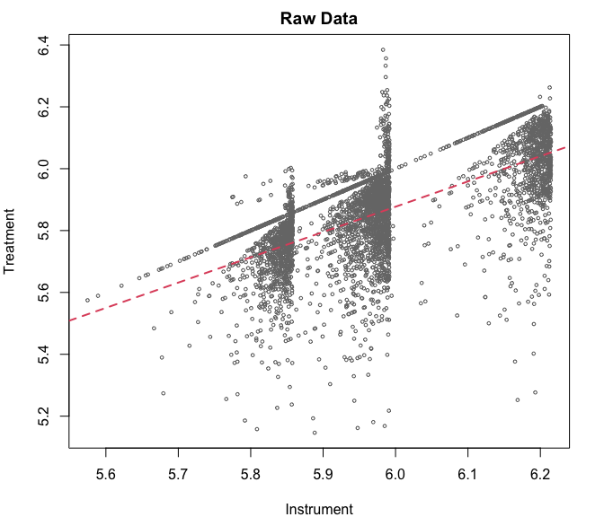
# first stage (partial out)
z_res <- lm(lz_pob_mesa_f ~ lpopulation + lpotencial, data = rueda)$residuals
d_res <- lm(lm_pob_mesa ~ lpopulation + lpotencial, data = rueda)$residuals
plot(z_res, d_res, col = "#777777", cex = 0.5,
     main = "Covariates Partialled Out",
     xlab = "Residualized Instrument",
     ylab = "Residualized Treatment")
abline(lm(d_res ~ z_res), col = 2, lwd = 2, lty = 2)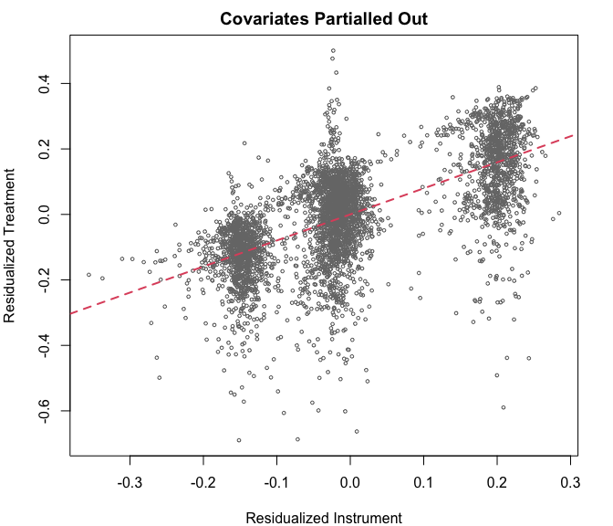
Omnibus function
The omnibus function ivDiag conducts both OLS and 2SLS
estimation and quantify uncertainties using multiple inferential
methods. It also output relevant information such as the first-stage
F-statistics and results from the AR test.
library(ivDiag)
g <- ivDiag(data = rueda, Y=Y, D = D, Z = Z, controls = controls, cl = cl)
names(g)
#>  [1] "est_ols"  "est_2sls" "AR"       "F_stat"   "rho"      "tF"
#>  [7] "est_rf"   "est_fs"   "p_iv"     "N"        "N_cl"     "df"
#> [13] "nvalues"
OLS estimation and inferential results
est_ols stores OLS results from the linear model
felm(Y ~ D + controls | 0 | FE, data = df, weights = weights, cluster = cl),
along with inferetial resutls based on analytic SEs and two
(block-)bootstrap methods: the coefficient method (bootstrap-c) and
t-ratio method (bootstrap-t).
g$est_ols
#>            Coef     SE       t CI 2.5% CI 97.5% p.value
#> Analytic -0.675 0.1011 -6.6803 -0.8731  -0.4770       0
#> Boot.c   -0.675 0.1030 -6.5548 -0.8923  -0.4891       0
#> Boot.t   -0.675 0.1011 -6.6803 -0.8400  -0.5101       0
2SLS estimation and inferential resutls
est_2sls stores 2SLS results using the
felm package, along with analytic SEs and two
bootstrapped SEs.
g$est_2sls
#>             Coef     SE       t CI 2.5% CI 97.5% p.value
#> Analytic -0.9835 0.1424 -6.9071 -1.2626  -0.7044       0
#> Boot.c   -0.9835 0.1410 -6.9758 -1.2647  -0.7244       0
#> Boot.t   -0.9835 0.1424 -6.9071 -1.2248  -0.7423       0
Two additional inferential methods are provided. AR
stores results from the AR test, including the test statistic, the
p-value, the 95% CI using the inversion method proposed by Chernozhukov and Hansen (2008), and whether the
CI is bounded. Note that if a CI is empty, we define
AR$bounded = FALSE.
g$AR
#> $Fstat
#>         F       df1       df2         p
#>   48.4768    1.0000 4350.0000    0.0000
#>
#> $ci.print
#> [1] "[-1.2626, -0.7073]"
#>
#> $ci
#> [1] -1.2626 -0.7073
#>
#> $bounded
#> [1] TRUE
tF stores results from the tF procedure based
on Lee et al. (2022). tF$cF
is the critical value for the valid t test adjusted based on
the effective F statistic. The CIs are constructed based on
tF$t, tF$SE, and tF$cF.
g$tF
#>         F        cF      Coef        SE         t    CI2.5%   CI97.5%   p-value
#> 8598.3264    1.9600   -0.9835    0.1424   -6.9071   -1.2626   -0.7044    0.0000
Charaterizing the first stage
F_stat stores various first-stage partial
F-statistics, which assess the strength of the instruments.
They include F statistic based classic analytic SEs, robust
SEs, cluster-robust SEs (if cl is supplied),
(blocked-)bootstrapped F statistic, and the effective F statistic (Olea and Pflueger 2013).
g$F_stat
#>  F.standard    F.robust   F.cluster F.bootstrap F.effective
#>    3106.387    3108.591    8598.326    8408.152    8598.326
rho stores the Pearson correlation coefficient between
the treatment and predicted treatment from the first stage regression
(all covariates are partialled out).
g$rho
#> [1] 0.6455
est_fs stores results from the first stage regression.
Both analytic and (block-)bootstrap SEs are recorded (boostrap-c). The
CIs are based on the bootstrap percentile method.
g$est_fs
#>                 Coef     SE p.value   SE.b CI.b2.5% CI.b97.5% p.value.b
#> lz_pob_mesa_f 0.7957 0.0086       0 0.0087   0.7804    0.8145         0
Other relevant information
est_rf stores results from the reduced form regression.
SEs and CIs are produced similarly as in est_fs.
g$est_rf
#>                  Coef     SE p.value   SE.b CI.b2.5% CI.b97.5% p.value.b
#> lz_pob_mesa_f -0.7826 0.1124       0 0.1118  -1.0127   -0.5731         0
p_iv stores the number of instruments. N
and N_cl store the number of observations and the number of
clusters used in the OLS and 2SLS regression, respectively.
df stores the degree of freedom left from the 2SLS
regression. The nvalues stores the unique values the
outcome Y, the treatment D, and each
instrument in Z in the 2SLS regression.
g$p_iv
#> [1] 1
g$N
#> [1] 4352
g$N_cl
#> [1] 1098
g$df
#> [1] 4348
g$nvalues
#>      e_vote_buying lm_pob_mesa lz_pob_mesa_f
#> [1,]            16        4118          3860
Moreover, users can turn off bootstrapping by setting
bootstrap = FALSE:
ivDiag(data = rueda, Y=Y, D = D, Z = Z, controls = controls,
            cl = cl, bootstrap = FALSE)
Coefficients and CIs plot
The plot_coef() function produces a coefficient plot for
both OLS and 2SLS estimates using different inferential methods. It also
shows the effective F-statistic, as well as the numbers of
observations and clusters. This plot is made by base R and
can be further altered by users.
In this example, the 2SLS estimate is slightly larger in magnitude than the OLS estimate. Various inferential methods of the OLS (or 2SLS) estimate, as shown by the multiple CIs, more of less agree with each other, suggesting robustness of the findings.
plot_coef(g)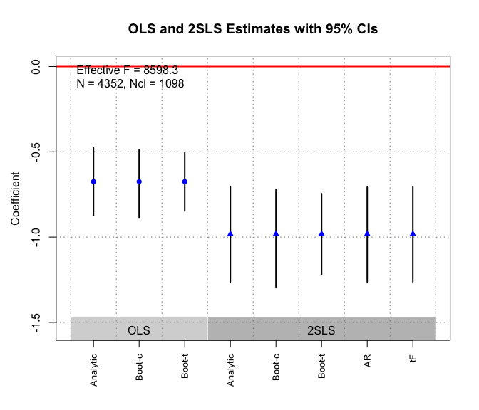
Users can also adjust the appearance of the plot and control which estimates to be shown using various options. For example:
plot_coef(g, ols.methods = c("analy"), iv.methods = c("analy", "ar", "tf"),
  main = "Comparison between OLS and IV Estimates", ylab = "Estimates",
  grid = FALSE, stats = FALSE, ylim = c(-2, 0.5))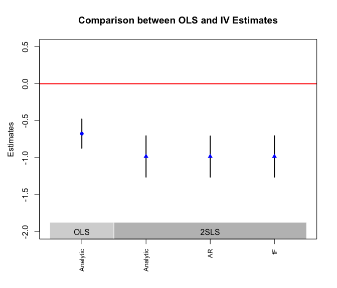
Conduct tests seperately
The ivDiag package also allows users to conduct
several important statistical tests seperately, including the effective
F statistic, the AR test, and the tF procedure. The
syntax of eff_F and AR_test are similar to
that of ivDiag.
Effective F statistic
eff_F(data = rueda, Y = Y, D = D, Z = Z, controls = controls, cl = cl,
      FE = NULL, weights = NULL)
#> [1] 8598.326
AR test
AR_test(data = rueda, Y = Y, D = D, Z = Z, controls = controls, cl = cl,
        FE = NULL, weights = NULL)
#> $Fstat
#>         F       df1       df2         p
#>   48.4768    1.0000 4350.0000    0.0000
#>
#> $ci.print
#> [1] "[-1.2626, -0.7073]"
#>
#> $ci
#> [1] -1.2626 -0.7073
#>
#> $bounded
#> [1] TRUE
tF procedure
tF takes in a 2SLS estimate, its SE (analytic or
bootstrapped), and the first-stage F statistics (obtained from
any methods).
tF(coef = -0.9835, se = 0.1540, Fstat = 8598)
#>         F        cF      Coef        SE         t    CI2.5%   CI97.5%   p-value
#> 8598.0000    1.9600   -0.9835    0.1540   -6.3864   -1.2853   -0.6817    0.0000
Sensitivity Tests
We also implement a set of sensitivity tests for researchers to gauge the validity of the exogeneity assumption, which is strong and generally untestable. Theses tests are applicable for the just-identified (one-treatment-one-instrument) case.
Bound and Jaeger (2000) suggest first using an auxiliary regression on a subsample where the instrument is not expected to influence treatment assignment, known as zero-first-stage (ZFS) tests. A ZFS test can be understood as a placebo test. The primary intuition is that in a subsample that one has a strong prior that the first stage is zero—-hence, they are never takers, to use the language of the LATE framework—the reduced form effect should also be zero if the assumption is satisfied. In other words, motivated by a substantive prior that the first-stage effect of the instrument is likely zero for a subsample of the population (henceforth, the ZFS subsample), the researcher then proceeds to show that the reduced-form coefficient for the instrument (by regression \(Y\) on \(Z\)) is approximately zero in the ZFS subsample, which is suggestive evidence in favor of instrument validity. Most observational instruments ought to yield some ZFS subsample based on substantive knowledge of the assignment mechanism.
While this is a useful heuristic check that we advise most observational IV papers adopt, it is an informal test and provides no test statistics. Van Kippersluis and Rietveld (2018) demonstrate that the ZFS test can be fruitfully combined with the “plausibly exogenous” method suggested by Conley, Hansen, and Rossi (2012) (henceforth, CHR 2012). To illustrate the method, we first rewrite the IV simultaneous equations in CHR (2012)’s notation:
\[ Y=X \beta+Z \gamma+\varepsilon ; \quad X=Z \Pi+v \]
where the instrument \(Z\) also enters the structural equation, the exclusion restriction amounts to a dogmatic prior that \(\gamma=0\). CHR (2012) suggest that this assumption can be relaxed, and replaced with a user-specified assumption on a plausible value, range, or distribution for \(\gamma\) depending on the researcher’s beliefs regarding the degree of exclusion restriction violation. They propose three different approaches for inference that involve specifying the range of values for \(\gamma\), a prior distributional assumption for \(\gamma\), and a fully Bayesian analysis that requires priors over all model parameters and corresponding parametric distributions. We focus on the second method, which CHR (2012) call the local-to-zero (LTZ) approximation because of its simplicity and transparency. The LTZ approximation considers “local” violations of the exclusion restriction and requires a prior over \(\gamma\) alone. CHR (2012) show that replacing the standard assumption that \(\gamma = 0\) with the weaker assumption that \(\gamma \sim \mathbb{F}\), a prior distribution, implies distribution for \(\hat\beta\) below: \[ \hat{\beta} \sim^a N(\beta, \mathbb{V}_{2SLS}) + A \gamma \] where \(A = X' Z (Z 'Z)^{-1} Z' X)^{-1} X'Z\) and the original 2SLS asymptotic distribution is inflated by the additional term. The distribution takes its most convenient form when one uses a Gaussian prior over \(\gamma \sim N(\mu_\gamma, \Omega_\gamma)\), which simplifies the above equation to the equation below, with a posterior being a Gaussian centered at \(\beta + A \mu_\gamma\). \[ \hat{\beta} \sim^a N(\beta + A \mu_\gamma , \mathbb{V}_{2SLS} + A \Omega A') \] In practice, researchers can replace \(\mu_\gamma\) with an estimate from the ZFS and \(\Omega\) with the estimate’s estimated variance.
The persistence of social captial
We illustrate the diagnostics by applying it to the IV analysis in Guiso, Sapienza, and Zingales (2016) (henceforth GSZ 2016), who revisit Putnam, Leonardi, and Nanetti (1992)’s celebrated conjecture that Italian cities that achieved self-government in the Middle Ages have higher modern-day levels of social capital. More specifically, they study the effects of free city-state status on social capital as measured by the number of nonprofit organizations and organ donations per capita, and a measure of whether students cheat in mathematics. Below is a summary. In this tutorial, we focus on the first outcome.
| Summary | |
|---|---|
| Unit of analysis | Italian city |
| Treatment | historical free city status |
| Instrument | whether a city was the seat of a bishop in the Middle Ages |
| Outcome | the number of nonprofit organizations per capita |
| Model | Table 6 |
Using the replication data, we first locate the key variables and take a look at the data. The outcome variable is highly skewed, but we keep it as is to be consistent with the original paper.
Y <- "totassoc_p"
D <- "libero_comune_allnord"
Z <- "bishopcity"
weights <- "population"
controls <- c('altitudine', 'escursione', 'costal', 'nearsea',
              'population', 'pop2', 'gini_land', 'gini_income')

# table instrument and treatment
table(gsz$bishopcity)
#>
#>    0    1
#> 5178  179
table(gsz$libero_comune_allnord)
#>
#>    0    1
#> 5293   64
table(gsz$bishopcity, gsz$libero_comune_allnord)
#>
#>        0    1
#>   0 5173    5
#>   1  120   59

# distribution of the outcome
hist(gsz$totassoc_p, breaks = 100,
     xlab = "# Nonprofit Organizations Per Capita")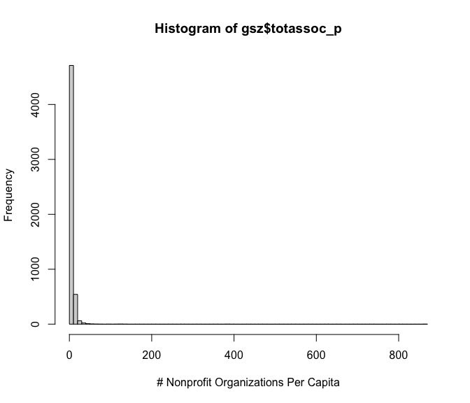
We apply omnibus function ivDiag and plot the OLS and
2SLS coefficients and corresponding CIs.
g <- ivDiag(data = gsz, Y = Y, D = D, Z = Z, controls = controls,
            weights = weights)
g
#> $est_ols
#>            Coef     SE      t CI 2.5% CI 97.5% p.value
#> Analytic 1.8317 0.3255 5.6266  1.1936   2.4697   0.000
#> Boot.c   1.8317 0.3642 5.0295  1.0153   2.4486   0.000
#> Boot.t   1.8317 0.3255 5.6266  1.0165   2.6468   0.001
#>
#> $est_2sls
#>            Coef     SE      t CI 2.5% CI 97.5% p.value
#> Analytic 4.2087 0.6670 6.3097  2.9014   5.5161       0
#> Boot.c   4.2087 0.8683 4.8472  2.5861   6.0501       0
#> Boot.t   4.2087 0.6670 6.3097  2.5588   5.8586       0
#>
#> $AR
#> $AR$Fstat
#>         F       df1       df2         p
#>   54.2805    1.0000 5355.0000    0.0000
#>
#> $AR$ci.print
#> [1] "[3.0481, 5.7429]"
#>
#> $AR$ci
#> [1] 3.0481 5.7429
#>
#> $AR$bounded
#> [1] TRUE
#>
#>
#> $F_stat
#>  F.standard    F.robust   F.cluster F.bootstrap F.effective
#>   1581.0235     67.3057          NA     52.0536     67.3057
#>
#> $rho
#> [1] 0.4777
#>
#> $tF
#>       F      cF    Coef      SE       t  CI2.5% CI97.5% p-value
#> 67.3057  2.0600  4.2087  0.6670  6.3097  2.8347  5.5828  0.0000
#>
#> $est_rf
#>              Coef    SE p.value  SE.b CI.b2.5% CI.b97.5% p.value.b
#> bishopcity 1.6124 0.219       0 0.269   0.9284    1.9678         0
#>
#> $est_fs
#>              Coef     SE p.value   SE.b CI.b2.5% CI.b97.5% p.value.b
#> bishopcity 0.3831 0.0467       0 0.0531   0.2634    0.4681         0
#>
#> $p_iv
#> [1] 1
#>
#> $N
#> [1] 5357
#>
#> $N_cl
#> NULL
#>
#> $df
#> [1] 5347
#>
#> $nvalues
#>      totassoc_p libero_comune_allnord bishopcity
#> [1,]       4545                     2          2
#>
#> attr(,"class")
#> [1] "ivDiag"
The results show that the 2SLS estimates are larger in magnitude than the OLS estimates. Different inferential methods for the 2SLS estimates produce slightly different CIs, but all reject the null of no effect quite comfortably.
plot_coef(g)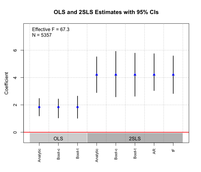
ZFS tests and LTZ adjustment
The authors conduct a ZFS test using the subsample of southern
Italian cities, where the free-city experience was arguably irrelevant.
The ZFS test is simply a reduced-form regression of the outcome on the
instrument. The coefficient and SE of the instrument
bishopcity is 0.178 and 0.137,
respectively.
library(estimatr)
zfs <- lm_robust(totassoc_p ~ bishopcity + altitudine + escursione
                 + costal + nearsea + population + pop2 + gini_land +
                   gini_income + capoluogo, data = gsz_south,
                 weights = gsz_south$population, se_type = "HC1")

summary(zfs)$coefficients["bishopcity", 1:2]
#>   Estimate Std. Error
#>  0.1778017  0.1373264
Setting 0.178 as the prior mean and 0.137
as its standard deviation (SD), we can perform a LTZ adjustment on the
2SLS/IV estimate.
ltz_out <- ltz(data = gsz, Y = Y, D = D, Z = Z,
controls = controls, weights = weights,
prior = c(0.178, 0.137))
ltz_out
#> $iv
#> Coef SE t CI 2.5% CI 97.5% p-value
#> 4.2087 0.6670 6.3097 2.9014 5.5160 0.0000
#>
#> $ltz
#> Coef SE t CI 2.5% CI 97.5% p-value
#> 3.6088 0.8112 4.4485 2.0188 5.1988 0.0000
#>
#> $prior
#> Mean SD
#> 0.178 0.137
#>
#> attr(,"class")
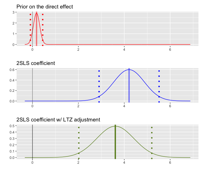
#> [1] "ltz"plot_ltz is a function that visualizes the approximated
sampling distribution of the 2SLS estimates before and after LTZ
adjustment, as well as the prior distribution formed based on the ZFS
test. It takes the output from the ltz function as input.
The dotted lines represent the 95% CIs. We see that, in this case, the
original finding remains robust to the LTZ adjustment.

plot_ltz can also take in the IV estimates, the LTZ
estimates, and the prior separately, all of which are two-element
vectors with a coefficient and a SD/SE estimate.
plot_ltz(iv_est = ltz_out$iv[1:2], ltz_est = ltz_out$ltz[1:2],
         prior = ltz_out$prior)