8 Conformal Inference
Suppose one state adopts a policy in 2010 and 45 states never do. We fit a factor model, predict the state’s outcome without the policy, and read the effect in each year as the gap between what happened and the prediction. How far off could that prediction be? The bootstrap and the jackknife answer by resampling treated units, and with one treated unit there is nothing to resample. The parametric bootstrap answers with a model of the prediction errors, which has to be right.
Conformal inference answers by comparison. Pretend, one at a time, that each of the 45 states had adopted the policy in 2010, predict it the same way, and look at how far off those predictions are. The treated state’s prediction error should look like one of theirs. If the largest of the 45 errors in 2012 is 2.4, it would be unusual for the treated state’s error in 2012 to be larger.
vartype = "conformal" (new in 2.4.9) turns this comparison into intervals, using the Jackknife+ of Liu and Xu (2026). It gives an interval for each treated unit and each date after treatment, with a coverage guarantee that holds in finite samples. It works with method = "gsynth", "ife" and "mc" when the treatment never switches off. For the fixed-effects model and for estimators such as synthetic control, fect also offers the paper’s full conformal inference (Section 8.7). This chapter explains the idea, says what the guarantee needs, and shows how to use it with one and with several treated units.
8.1 The idea
Take one treated unit and one date after treatment. The never-treated units, called controls below, are paired with the treated unit one at a time. In the fold for control \(j\):
- Both units hide their outcomes from the treated unit’s adoption date on. Control \(j\) keeps only the treated unit’s pre-treatment window, so it is predicted from the same amount of history.
- The other controls keep their full panels. Each hidden unit is predicted from them, in a separate fit.
- Control \(j\) was never treated, so its outcome at the date is known. Its prediction error \(R_j\) shows how far off a prediction from this fold can be.
- The fold gives the treated unit’s prediction \(\hat M_{0j}\) and two endpoints, \(\hat M_{0j} - R_j\) and \(\hat M_{0j} + R_j\).
With \(J\) controls there are \(J\) folds and \(J\) pairs of endpoints. Let \(N = J + 1\), the controls plus the treated unit. The interval for the treated unit’s untreated outcome runs from the \(q\)-th smallest lower endpoint to the \(q\)-th largest upper endpoint, where \(q\) is the largest integer with \((2q - 1)/N \le\) alpha. Subtracting the interval from the observed outcome gives the interval for the effect.
The interval covers the effect with probability at least \(1 - (2q - 1)/N\). Two examples:
- With 19 controls and
alpha = 0.1, \(N = 20\) and \(q = 1\). The interval runs from the smallest lower endpoint to the largest upper one, and the guarantee is \(1 - 1/20 = 0.95\). - With 45 controls and
alpha = 0.1, \(N = 46\) and \(q = 2\). The second smallest and second largest endpoints are used, and the guarantee is \(1 - 3/46 = 0.935\).
The guarantee is at least \(1 -\) alpha and can be higher, because \(N\) is a whole number. With fewer than \(1/\)alpha \(- 1\) controls, \(q = 0\) and the interval is the whole real line: there are too few controls to tell an unusual error from a usual one. Each interval also has a p-value for the null of no effect at that date. It is at most alpha exactly when the interval excludes zero, and it can be no smaller than \(1/N\).
8.2 What the guarantee needs
The guarantee rests on a comparison, so it needs the comparison to be fair.
- The treated unit is no harder to predict than the controls. Formally, take the table of pair errors, whose entry for units \(i\) and \(k\) is unit \(i\)’s error when the two are held out together. Its distribution must not change when the units are relabeled. The usual way this fails is a treated unit unlike any control, for example one whose factor loadings lie outside the controls’ range. Its prediction is then an extrapolation, and its errors can be larger than any control’s.
-
The tuning is fixed in advance. Every fold reuses the original fit’s number of factors
r(orlambdafor"mc"). If that number was chosen by cross-validation, the choice depends on the data in ways that can favor one group. See Section 8.8. - No anticipation and no reversal. Outcomes before adoption are untreated, and treatment stays on once it starts.
-
Enough controls. About \(1/\)
alphaor more never-treated units, as above.
The guarantee does not need the factor model to be correct, the errors to be stationary, or a long pre-treatment period. A poor model makes the intervals wider. They keep their guarantee as long as the model is equally poor for the treated unit and the controls. fect cannot check the first two conditions. Section 8.5 shows how to look for evidence against the first.
8.3 One treated unit
We start with the synthetic control setting. sim_gsynth, from Chapter 6, has five treated units, 45 never-treated controls, 30 periods and two factors. We keep the first treated unit and the 45 controls.
The call is a usual gsynth fit with three changes: vartype = "conformal", a single number of factors with CV = FALSE, and alpha set to the error rate we accept.
out.cf1 <- fect(Y ~ D + X1 + X2, data = d1, index = c("id", "time"),
                method = "gsynth", force = "two-way", r = 2, CV = FALSE,
                se = TRUE, vartype = "conformal", alpha = 0.1)
#>
#>  +----------------------------------------------------------+
#>  | Parallel computing: using 8 of 20 available cores.       |
#>  |                                                          |
#>  | To change: set cores = <n> in fect().                    |
#>  | Default: min(available - 2, 8).                          |
#>  +----------------------------------------------------------+
print(out.cf1)
#> Call:
#> fect.formula(formula = Y ~ D + X1 + X2, data = d1, index = c("id",
#>     "time"), force = "two-way", r = 2, CV = FALSE, method = "gsynth",
#>     se = TRUE, vartype = "conformal", alpha = 0.1)
#>
#> Estimator:    gsynth
#> Fixed effects: id (unit) + time (time)
#> Inference:     conformal, Jackknife+ for full-path estimators (90% level; 45 never-treated controls; no S.E.)
#>
#> ATT:
#>                             ATT S.E. CI.lower CI.upper p.value
#> Tr obs equally weighted   5.701   NA    4.552    6.877 0.02174
#> Tr units equally weighted 5.701   NA    4.552    6.877 0.02174
#>
#> Covariates:
#>     Coef S.E. CI.lower CI.upper p.value
#> X1 1.021   NA       NA       NA      NA
#> X2 3.052   NA       NA       NA      NA
The intervals for each date are in out.cf1$conformal$unit. The columns N and q give the pool size and the endpoint used.
cu1 <- out.cf1$conformal$unit
cu1[, c("time", "event.time", "eff", "CI.lower", "CI.upper", "p.value", "N", "q")]
#>    time event.time       eff   CI.lower  CI.upper    p.value  N q
#> 1    21          1 0.3427166 -2.8477403  3.517339 1.00000000 46 2
#> 2    22          2 4.3293409  2.3030170  6.702014 0.02173913 46 2
#> 3    23          3 4.3050815  1.8901546  6.636109 0.02173913 46 2
#> 4    24          4 3.6521716  0.8933277  6.393756 0.06521739 46 2
#> 5    25          5 4.8472393  2.6269154  7.110497 0.02173913 46 2
#> 6    26          6 4.5927316  2.3517049  6.935179 0.02173913 46 2
#> 7    27          7 8.6253924  6.5457063 10.599441 0.02173913 46 2
#> 8    28          8 8.1855355  5.4379757 11.085550 0.02173913 46 2
#> 9    29          9 8.9644704  6.8044102 11.000078 0.02173913 46 2
#> 10   30         10 9.1701093  6.7033030 11.576206 0.02173913 46 2
Read the second row. At the second period after treatment, the estimated effect is 4.33 and the interval runs from 2.3 to 6.7. With \(N = 46\) and \(q = 2\), it covers the effect with probability at least 0.935 if the conditions above hold. Its p-value, 0.022, equals \(1/46\), the smallest possible with 45 controls. The interval for the first period includes zero.
The gap plot draws the same intervals, since with one treated unit the average effect at each event time is that unit’s effect.
plot(out.cf1, main = "One treated unit, conformal intervals")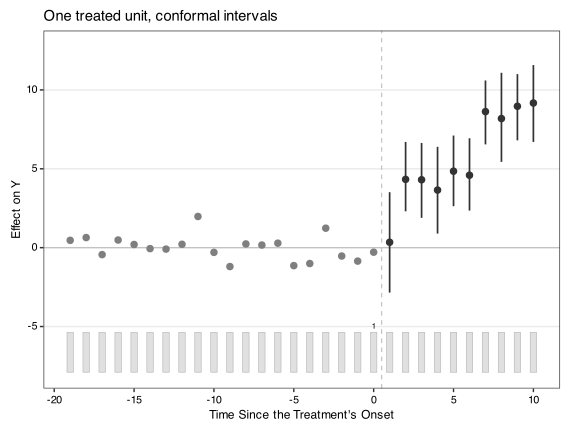
Each interval has its guarantee at its own date. They are not joint: across the ten dates, about one interval in ten can miss by chance. est.avg also reports an interval for the average effect over the ten dates. With one treated unit, Liu and Xu (2026) cover such averages over dates, with the same conditions.
8.4 Several treated units
Now we use all five treated units.
out.cf <- fect(Y ~ D + X1 + X2, data = sim_gsynth, index = c("id", "time"),
               method = "gsynth", force = "two-way", r = 2, CV = FALSE,
               se = TRUE, vartype = "conformal", alpha = 0.1)
#>
#>  +----------------------------------------------------------+
#>  | Parallel computing: using 8 of 20 available cores.       |
#>  |                                                          |
#>  | To change: set cores = <n> in fect().                    |
#>  | Default: min(available - 2, 8).                          |
#>  +----------------------------------------------------------+
print(out.cf)
#> Call:
#> fect.formula(formula = Y ~ D + X1 + X2, data = sim_gsynth, index = c("id",
#>     "time"), force = "two-way", r = 2, CV = FALSE, method = "gsynth",
#>     se = TRUE, vartype = "conformal", alpha = 0.1)
#>
#> Estimator:    gsynth
#> Fixed effects: id (unit) + time (time)
#> Inference:     conformal, Jackknife+ for full-path estimators (90% level; 45 never-treated controls; no S.E.)
#> Aggregates:    intervals for averages over 5 treated units have no coverage guarantee (?fect)
#>
#> ATT:
#>                             ATT S.E. CI.lower CI.upper p.value
#> Tr obs equally weighted   5.543   NA    4.399    6.728 0.02174
#> Tr units equally weighted 5.543   NA    4.399    6.728 0.02174
#>
#> Covariates:
#>     Coef S.E. CI.lower CI.upper p.value
#> X1 1.021   NA       NA       NA      NA
#> X2 3.052   NA       NA       NA      NA
8.4.1 An interval for each unit and date
Each treated unit gets its own intervals, built against the same 45 controls as before. Under the conditions above, each covers that unit’s effect at that date with probability at least 0.935.
library(ggplot2)
cu <- out.cf$conformal$unit
ggplot(cu, aes(x = event.time, y = eff)) +
  geom_hline(yintercept = 0, linetype = "dashed", colour = "grey50") +
  geom_pointrange(aes(ymin = CI.lower, ymax = CI.upper), size = 0.2) +
  facet_wrap(~ unit, nrow = 1) +
  scale_x_continuous(breaks = seq(2, 10, by = 2)) +
  labs(x = "Periods since treatment", y = "Effect on Y") +
  theme_bw()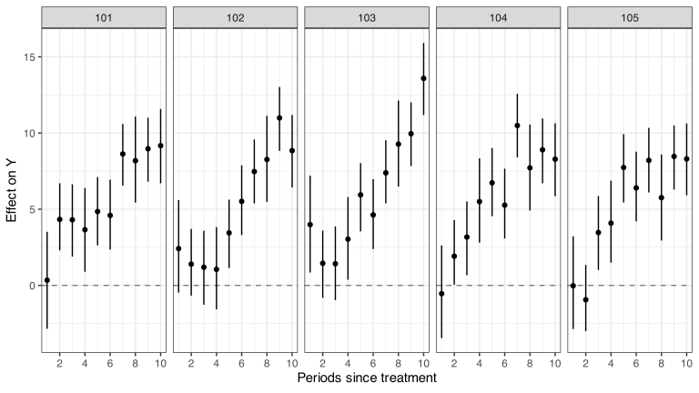
8.4.2 Block Jackknife+ for the average effect
For the average effect over the treated units, use the block Jackknife+ of Liu and Xu (2026). Without conformal.block = TRUE, the fit above also reports intervals for averages in est.att, est.avg and the gap plot, but these intervals have no guarantee, and we do not recommend reporting them. They compare an average of five treated units’ errors with one control’s error, and the average is usually less noisy. In a constructed example in ?fect, such an interval covers the average effect with probability 0.42 at a nominal 0.90. print() and the caption of the gap plot say so.
The block Jackknife+ compares like with like: the five treated units, taken together, against blocks of five controls. conformal.block = TRUE does the following.
- It splits the 45 controls at random into nine blocks of five.
- Within each block, each control is matched with one treated unit and takes that unit’s pre-treatment window and adoption date.
- Each fold hides the treated units and one block from their adoption dates on, and fits the model once.
- The fold’s prediction for the average is the average of the treated units’ predictions. Its score is the absolute average error of the block’s five controls at the same dates.
The interval then follows the rule in Section 8.1, with the nine blocks in place of the 45 controls: \(N = 9 + 1 = 10\), \(q = 1\) at alpha = 0.1, and the guarantee is \(1 - 1/10 = 0.9\).
The guarantee holds for the average effect even when effects differ across the treated units. It needs the treated units, as a block, to be as easy to predict as a block of controls. A finite interval at alpha = 0.1 needs at least nine controls per treated unit, and controls with missing outcomes stay out of the blocks. The partition is random, so set seed to reproduce it. With staggered adoption, each control takes its matched unit’s adoption date, and the average at an event time uses the treated units observed then and their matched controls.
The fit below also adds the pre-treatment diagnostics and the relabeling test, which the next two sections explain.
out.cfb <- fect(Y ~ D + X1 + X2, data = sim_gsynth, index = c("id", "time"),
                method = "gsynth", force = "two-way", r = 2, CV = FALSE,
                se = TRUE, vartype = "conformal", alpha = 0.1,
                conformal.block = TRUE, conformal.diag = 4,
                conformal.relabel = 999, seed = 1234)
#>
#>  +----------------------------------------------------------+
#>  | Parallel computing: using 8 of 20 available cores.       |
#>  |                                                          |
#>  | To change: set cores = <n> in fect().                    |
#>  | Default: min(available - 2, 8).                          |
#>  +----------------------------------------------------------+
print(out.cfb)
#> Call:
#> fect.formula(formula = Y ~ D + X1 + X2, data = sim_gsynth, index = c("id",
#>     "time"), force = "two-way", r = 2, CV = FALSE, method = "gsynth",
#>     se = TRUE, vartype = "conformal", alpha = 0.1, seed = 1234,
#>     conformal.diag = 4, conformal.block = TRUE, conformal.relabel = 999)
#>
#> Estimator:    gsynth
#> Fixed effects: id (unit) + time (time)
#> Inference:     conformal, Jackknife+ for full-path estimators (90% level; 45 never-treated controls; no S.E.)
#> Aggregates:    block Jackknife+, 9 control blocks of 5 (N = 10, q = 1)
#> Diagnostics:   last 4 pre-treatment dates; 1 of 20 unit-date intervals exclude zero
#> Relabeling:    sharp null of no effect, 999 draws, p = 0.001 (absolute average effect)
#>
#> ATT:
#>                             ATT S.E. CI.lower CI.upper p.value
#> Tr obs equally weighted   5.543   NA    5.026    5.983     0.1
#> Tr units equally weighted 5.543   NA    5.026    5.983     0.1
#>
#> Covariates:
#>     Coef S.E. CI.lower CI.upper p.value
#> X1 1.021   NA       NA       NA      NA
#> X2 3.052   NA       NA       NA      NA
The partition is in out.cfb$conformal$block$partition. In the gap plot, the intervals after treatment are block Jackknife+ intervals, and the four dates before treatment show the diagnostics.
plot(out.cfb, main = "Average effect, block Jackknife+ intervals")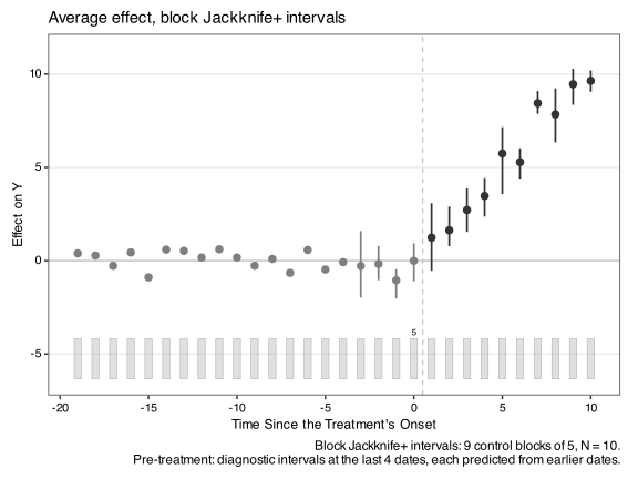
8.5 Checking the assumption
The guarantee needs the treated units to be no harder to predict than the controls. No test can prove this, but two checks can find evidence against it.
8.5.1 Where the treated units’ loadings lie
With a factor model, a treated unit whose loadings lie far from the controls’ is predicted by extrapolation. The loading.overlap plot from Chapter 6 shows the control loadings, their convex hull, and the treated units’ loadings. Treated units inside or near the hull are the comfortable case.
plot(out.cf, type = "loading.overlap")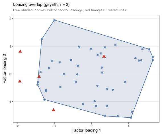
In this fit, three of the five treated units lie outside the hull, to the left of the controls. Their intervals depend more on the condition that they are no harder to predict than the controls, so their pre-treatment diagnostics deserve a close look.
8.5.2 Pre-treatment diagnostics
conformal.diag = 4 runs the procedure at each treated unit’s last four dates before treatment, as if the unit had adopted then. Its outcomes from that date on are hidden, and the outcome at the date is predicted from earlier dates and the controls. The estimate is a pseudo-effect, which should be zero, since nothing had happened yet. The interval and p-value test that zero. An interval away from zero says the unit was harder to predict than the controls before treatment, which weakens the case for the intervals after it.
du <- out.cfb$conformal$diag$unit
head(du[, c("unit", "time", "event.time", "eff", "CI.lower", "CI.upper",
            "p.value")], 8)
#>   unit time event.time        eff  CI.lower CI.upper   p.value
#> 1  101   17         -3  2.0981678 -1.678842 5.955015 0.4565217
#> 2  101   18         -2 -0.5887524 -2.584660 1.268759 0.9782609
#> 3  101   19         -1 -1.0596333 -3.275151 1.186297 0.6739130
#> 4  101   20          0 -0.4884469 -2.997973 1.945510 1.0000000
#> 5  102   17         -3  0.3834513 -3.484942 4.048739 1.0000000
#> 6  102   18         -2  0.8564613 -1.169866 2.664442 0.6304348
#> 7  102   19         -1 -0.6388171 -2.918705 1.542744 1.0000000
#> 8  102   20          0 -0.9348553 -3.407044 1.536439 0.8043478
The dates are not adjusted for multiple testing. At alpha = 0.1, about \(0.1 \times 4 = 0.4\) of each unit’s four intervals are expected to exclude zero by chance, so one miss is no cause for alarm and a run of misses is. The pre-treatment rows of est.att hold the average pseudo-effect at each of the four event times, with the same kind of interval as the rows after treatment (block Jackknife+ here).
8.6 Testing for any effect
The intervals ask how large the effect is at each date. The relabeling test asks a simpler question: did the treatment have any effect at all? Under the sharp null of no effect in any treated cell, every observed outcome is untreated, and the treated units are just five units with adoption dates attached.
conformal.relabel = 999 gives the five adoption dates to five units drawn at random, 999 times, refits the model each time, and records the average effect over the new treated cells. The p-value is the share of the 1,000 assignments, the actual one included, whose absolute average effect is at least as large as the actual one. It is exact if the treated units, absent treatment, are as easy to predict as any five other units. With random assignment, it is Fisher’s randomization test.
Here the p-value is 0.001, the smallest possible with 999 draws. The same draws give a p-value at each event time, in out.cfb$conformal$relabel$att. The plot shows each draw’s average effect by period in grey and the actual one in blue. It is the placebo plot of the synthetic control literature, with five units moved at a time.
rl <- out.cfb$conformal$relabel
paths <- data.frame(
  event.time = rep(as.numeric(rownames(rl$paths)), ncol(rl$paths)),
  eff = c(rl$paths),
  draw = rep(seq_len(ncol(rl$paths)), each = nrow(rl$paths))
)
ggplot(paths, aes(x = event.time, y = eff, group = draw)) +
  geom_line(colour = "grey80", linewidth = 0.3) +
  geom_hline(yintercept = 0, linetype = "dashed", colour = "grey50") +
  geom_line(data = rl$att, aes(x = event.time, y = ATT), inherit.aes = FALSE,
            colour = "#004a8c", linewidth = 1) +
  scale_x_continuous(breaks = seq(2, 10, by = 2)) +
  labs(x = "Periods since treatment", y = "Average effect on Y") +
  theme_bw()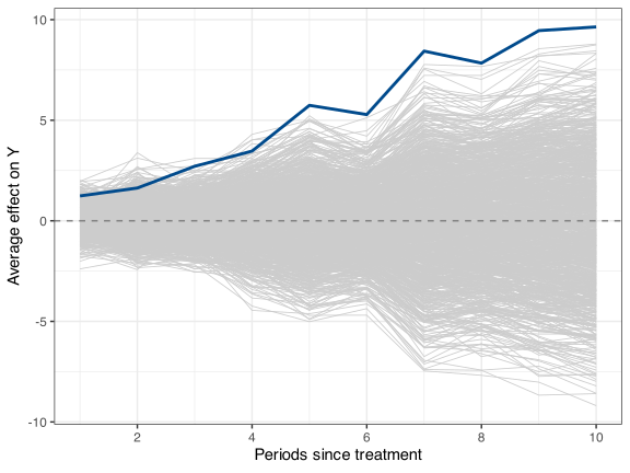
8.7 Full conformal inference for target-date estimators
The estimators used so far, "gsynth", "ife" and "mc", fit the whole panel, so their prediction for one date can use the controls’ outcomes at every date after treatment. Liu and Xu (2026) call them full-path estimators. A target-date estimator predicts the treated unit at a date from pre-treatment outcomes and the controls’ outcomes at that date only. Synthetic control is one: its weights come from the pre-treatment path, and it applies them to the controls’ outcomes at the date. So is the two-way fixed-effects imputation of method = "fe" with one treated unit and controls observed at every date. Its prediction is the treated unit’s pre-treatment mean plus the controls’ average change from their pre-treatment means to the date.
For target-date estimators the paper gives a second procedure, full conformal inference, and recommends it. It tests each candidate effect \(c\) in turn:
- Set the treated unit’s untreated outcome at the date to its observed outcome minus \(c\). If \(c\) is the true effect, the panel now holds only untreated outcomes.
- Hold out each unit alone, the treated unit included, and predict its outcome at the date from all the others. A control’s prediction uses the treated unit’s completed outcome. The treated unit’s prediction is the ordinary estimate, so its error is \(\hat\tau - c\).
- The p-value of \(c\) is the share of units whose absolute error is at least the treated unit’s. The set keeps the candidates with p-value above
alpha.
If the errors are exchangeable at the true effect, the set covers it with probability at least \(1 - \lfloor \alpha N \rfloor / N\), which is at least \(1 -\) alpha: with 45 controls and alpha = 0.1, \(N = 46\) and the guarantee is \(1 - 4/46 = 0.913\). The Jackknife+ guarantee for the same \(N\) is \(1 - 3/46 = 0.935\), but in the paper’s simulations full conformal sets are narrower where the Jackknife+ covers more than it promises. For the fixed-effects rule and for synthetic control, each unit’s error is a straight-line function of \(c\), so fect finds the set exactly, with no grid of candidates. For these two estimators the set is always one interval, because every control’s weight on the treated unit lies between 0 and 1. A rule written by the user can put a larger weight on it, and then the set can be a union of intervals; CI.lower and CI.upper give its hull, and disconnected is TRUE.
8.7.1 With the fixed-effects model
vartype = "conformal" with method = "fe" runs full conformal inference. We use the one-treated-unit data from Section 8.3.
out.fe <- fect(Y ~ D, data = d1, index = c("id", "time"), method = "fe",
               se = TRUE, vartype = "conformal", alpha = 0.1,
               conformal.diag = 4)
#>
#>  +----------------------------------------------------------+
#>  | Parallel computing: using 8 of 20 available cores.       |
#>  |                                                          |
#>  | To change: set cores = <n> in fect().                    |
#>  | Default: min(available - 2, 8).                          |
#>  +----------------------------------------------------------+
print(out.fe)
#> Call:
#> fect.formula(formula = Y ~ D, data = d1, index = c("id", "time"),
#>     method = "fe", se = TRUE, vartype = "conformal", alpha = 0.1,
#>     conformal.diag = 4)
#>
#> Estimator:    fe
#> Fixed effects: id (unit) + time (time)
#> Inference:     conformal, full conformal for target-date estimators (difference in differences rule; 91.3% level or higher; 45 never-treated controls; no S.E.)
#> Diagnostics:   last 4 pre-treatment dates; 0 of 4 unit-date intervals exclude zero
#> EM convergence: stopped by tol after 1 rounds (final relative change 4.818e-16, tol = 1e-05)
#>
#> ATT:
#>                             ATT S.E. CI.lower CI.upper p.value
#> Tr obs equally weighted   5.941   NA   0.5094    11.31 0.06522
#> Tr units equally weighted 5.941   NA   0.5094    11.31 0.06522
head(out.fe$conformal$unit[, c("time", "event.time", "eff", "CI.lower",
                                "CI.upper", "p.value", "N")])
#>   time event.time       eff    CI.lower  CI.upper   p.value  N
#> 1   21          1  4.085783  -5.4506140 13.291134 0.5869565 46
#> 2   22          2 -1.134195 -16.0408304 13.909271 0.9565217 46
#> 3   23          3 -3.141066 -12.7801617  6.078939 0.6304348 46
#> 4   24          4  9.243183  -0.4981143 19.427266 0.1086957 46
#> 5   25          5  6.611005  -4.1005956 17.090406 0.3695652 46
#> 6   26          6  5.491168  -1.1539055 11.901307 0.2173913 46
With one treated unit the event-time rows of est.att are its sets at each date, and est.avg is the set for its effect averaged over the post-treatment dates. The gap plot draws them, with the pre-treatment diagnostics at the last four dates before treatment.
plot(out.fe, main = "Fixed effects, full conformal sets")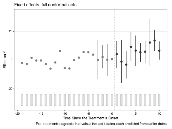
These sets are wide because the fixed-effects model leaves out the two factors that drive sim_gsynth. The guarantee still holds if the treated unit is no harder to predict than the controls under that model, but the sets reflect how poorly the model predicts. With several treated units, fect reports a set for each unit and date (and each unit’s average over its dates) in fit$conformal$unit and fit$conformal$avg, and the averages over units in est.att and est.avg carry no interval. With staggered adoption, each treated unit is compared with the never-treated units over its own pre-treatment dates, and fect says when this target-date estimate differs from its ordinary estimate.
8.7.2 Synthetic control and other estimators: conformal_sc()
conformal_sc() gives conformal inference for synthetic control and other target-date estimators. The estimator is a rule: "sc" (the default: synthetic control with simplex weights fitted on the pre-treatment outcomes; it needs the quadprog package), "did" (the fixed-effects rule above), or a function the user writes. The procedure is the user’s choice: procedure = "full" (the default) for full conformal sets, or procedure = "jackknife+" for Jackknife+ intervals. On Proposition 99 and German reunification, it reproduces the paper’s synthetic control results.
out.sc <- conformal_sc(Y ~ D, data = d1, index = c("id", "time"),
                       alpha = 0.1, diag = 4)
print(out.sc)
#> Call:
#> conformal_sc(formula = Y ~ D, data = d1, index = c("id", "time"),
#>     alpha = 0.1, diag = 4)
#>
#> Full conformal inference (Liu and Xu 2026), rule: sc (ridge-simplex, eta = 1e-05), alpha = 0.1
#> Treated units: 1; never-treated controls: 45
#> Guaranteed coverage of each date's set: 0.913
#>
#> By unit and date:
#>  unit time event.time    eff CI.lower CI.upper p.value  N
#>   101   21          1 -0.454   -8.734     7.99  0.9565 46
#>   101   22          2 -4.534  -12.039     2.97  0.3261 46
#>   101   23          3 -3.843  -12.282     4.59  0.4348 46
#>   101   24          4  7.526    1.028    14.02  0.0435 46
#>   101   25          5  4.179   -2.002    10.36  0.3261 46
#>   101   26          6  5.201   -0.343    10.75  0.1522 46
#>   101   27          7  3.914   -3.502    11.33  0.4130 46
#>   101   28          8  7.829   -0.994    16.65  0.1304 46
#>   101   29          9 10.765    4.871    16.66  0.0217 46
#>   101   30         10  6.770    1.310    12.23  0.0652 46
#>
#> Average over the post-treatment dates, by unit:
#>  unit n.dates  eff CI.lower CI.upper p.value  N
#>   101      10 3.74    0.768      6.7  0.0652 46
#>
#> Pre-treatment placebo dates: 0 of 4 sets exclude zero
out.sc$unit holds the set for each date, out.sc$avg the set for the effect averaged over the post-treatment dates (its guarantee needs the units’ errors averaged over the dates to be exchangeable), and out.sc$diag the pre-treatment placebo dates. plot(out.sc) draws them.
plot(out.sc)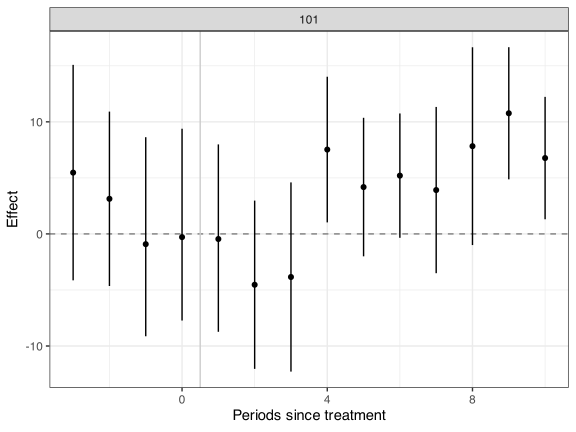
The same rule with procedure = "jackknife+" gives Jackknife+ intervals. Both procedures have a guarantee under the same conditions. For a target-date estimator the paper recommends full conformal inference: its sets cover at their stated level, while Jackknife+ intervals often cover more than they state and are then wider. The Jackknife+ is the better choice when the rule is not a straight-line function of the outcomes, since full conformal inference then needs a grid of candidates and a refit of every control at each one. The table below compares the two for the synthetic control fit above.
out.jp <- conformal_sc(Y ~ D, data = d1, index = c("id", "time"),
                       procedure = "jackknife+", alpha = 0.1)
cmp <- data.frame(event.time = out.sc$unit$event.time,
                  full.lower = out.sc$unit$CI.lower,
                  full.upper = out.sc$unit$CI.upper,
                  jackknife.lower = out.jp$unit$CI.lower,
                  jackknife.upper = out.jp$unit$CI.upper)
round(cmp, 2)
#>    event.time full.lower full.upper jackknife.lower jackknife.upper
#> 1           1      -8.73       7.99           -9.81           10.45
#> 2           2     -12.04       2.97          -13.58            5.41
#> 3           3     -12.28       4.59          -13.52            5.83
#> 4           4       1.03      14.02            0.18           14.87
#> 5           5      -2.00      10.36           -2.47           10.83
#> 6           6      -0.34      10.75           -1.25           11.66
#> 7           7      -3.50      11.33           -4.60           12.94
#> 8           8      -0.99      16.65           -2.53           18.18
#> 9           9       4.87      16.66            4.40           17.58
#> 10         10       1.31      12.23           -0.20           13.33
c(full = out.sc$unit$level[1], jackknife = out.jp$unit$level[1])
#>      full jackknife
#> 0.9130435 0.9347826
The last line gives each procedure’s guaranteed coverage with 45 controls: \(1 - 4/46 = 0.913\) for full conformal inference and \(1 - 3/46 = 0.935\) for the Jackknife+.
A user-written rule is a function of three arguments: the held-out unit’s outcomes at the pre-treatment dates, the training units’ outcomes at those dates (one column per unit), and the training units’ outcomes at the target date. It returns the held-out unit’s prediction at the target date, which it cannot see. The rule below shifts the training units’ mean at the date by the held-out unit’s average pre-treatment gap to them.
my_rule <- function(query.pre, background.pre, background.target) {
  mean(background.target) + mean(query.pre - rowMeans(background.pre))
}
out.my <- conformal_sc(Y ~ D, data = d1, index = c("id", "time"),
                       rule = my_rule, alpha = 0.1)
head(out.my$unit[, c("time", "eff", "CI.lower", "CI.upper", "method")])
#>   time       eff    CI.lower  CI.upper method
#> 1   21  4.085783  -5.4506140 13.291134  exact
#> 2   22 -1.134195 -16.0408304 13.909271  exact
#> 3   23 -3.141066 -12.7801617  6.078939  exact
#> 4   24  9.243183  -0.4981143 19.427266  exact
#> 5   25  6.611005  -4.1005956 17.090406  exact
#> 6   26  5.491168  -1.1539055 11.901307  exact
For a user-written rule, fect checks numerically whether the prediction is a straight-line function of the completed outcome: at five candidates far on both sides of zero, and again by refitting just inside and just outside the ends of the set. If both checks pass, the set is exact (method is "exact"). If not, the p-value is evaluated on a grid of candidates (grid), each of which refits every control; the set’s ends are as fine as the grid, and lower.truncated or upper.truncated flags a set that reaches the grid’s end. The guarantee needs the same conditions as before: the treated unit is no harder to predict than the controls under the rule, and the rule and its tuning, such as a synthetic control penalty, are fixed in advance and the same for every unit.
8.8 Tuning
All of these guarantees assume that the tuning is fixed in advance. Every fold, diagnostic, block and relabeling fit reuses the original fit’s number of factors or lambda. With CV = TRUE, that value is chosen from the data. With method = "gsynth", the default cross-validation scores the never-treated units’ held-out cells only. With "ife" and "mc", it also scores the treated units’ pre-treatment cells. Either way, the choice can fit the controls, or the treated units, better than the other group, and the guarantee no longer follows. fect then prints a message that names the chosen value.
No extra option is needed. Pass a single number of factors (or lambda) with CV = FALSE, as in the examples above. When the number of factors is unknown, it should be chosen before looking at the outcomes, for example from theory or from an earlier study, and reported. Choosing it by cross-validation on the controls alone does not help: that choice also favors one group. With few treated units, it is also worth showing that the conclusions hold for a nearby value.
8.9 Conformal or parametric bootstrap?
Both are meant for few treated units. They answer different questions and rest on different conditions.
| Parametric bootstrap | Conformal (Jackknife+) | |
|---|---|---|
| Output | Standard errors and intervals for the average effect by period and overall | Intervals for each treated unit and date; averages through the block Jackknife+ |
| Guarantee | Approximate, as the numbers of controls and pre-treatment periods grow | Finite-sample, at each date |
| Main conditions | The factor model holds for every unit, r is at least the true number of factors, the controls’ loadings span the factors, and errors are independent across units with the same distribution for treated units and controls |
The treated units are no harder to predict than the controls, the tuning is fixed, and there are about \(1/\)alpha or more controls |
| Methods |
"gsynth", and "ife" or "cfe" with time.component.from = "nevertreated"
|
"gsynth", "ife", "mc"
|
| Tuning by cross-validation | Allowed | Breaks the guarantee |
When both are possible, they can be reported side by side. If they disagree, the parametric intervals lean on the model of the errors, and the conformal intervals lean on the comparison with the controls. Chapter 7 explains the parametric bootstrap and its conditions.
8.10 Limits
- There are no standard errors.
S.E.isNA, andci.methoddoes not apply. - Full conformal inference (Section 8.7) covers target-date estimators only:
method = "fe"without covariates, and the rules given toconformal_sc(). - At least two never-treated units are needed, and about \(1/\)
alphaof them for a finite interval. - The diagnostics refit for each of their dates, and the relabeling test refits once per draw. With
"ife"and"mc", which fit once per held-out unit,conformal.diag = 4makes the run about five times longer. -
vartype = "conformal"stops with weights,group,balance.period, placebo and carryover tests,loo, permutation tests,cm, extra fixed effects, binary outcomes,loading.boundand treatments that switch off. The equivalence plot,estimand(),att.cumu(),effect()andfect_sens()need bootstrap draws and stop for these fits. - A fold fit that fails keeps its control in the pool with an infinite score. The interval widens,
Nandqdo not change, andfectwarns. See?fectfor the details.
8.11 Summary
A typical analysis with few treated units:
- Choose
r(orlambda) before looking at the outcomes after treatment, and fit withCV = FALSE. - Fit with
vartype = "conformal". With more than one treated unit, addconformal.block = TRUEfor the average effect, and setseed. - Add
conformal.diag = 4and look at the pre-treatment intervals and theloading.overlapplot. - Add
conformal.relabel = 999to test whether there is any effect. - With a target-date estimator, such as the fixed-effects model with one treated unit or synthetic control, use full conformal inference:
method = "fe"infect(), orconformal_sc(). - Report the intervals for each unit and date, the block interval for the average, the guarantee level (
print()shows it), and the diagnostics.
8.12 How to cite
Cite Liu and Xu (2026) for conformal inference in fect.
@misc{liuxu2026conformal,
  title = {Unit-Level Conformal Inference for Panel Counterfactuals},
  author = {Liu, Ziyi and Xu, Yiqing},
  year = {2026},
  eprint = {2611.19209},
  archivePrefix = {arXiv},
  url = {https://arxiv.org/abs/2611.19209}
}