
4 Factor-Based Methods
When the parallel trends assumption is violated due to latent common factors with heterogeneous loadings, the FE estimator from Chapter 2 is biased. This chapter introduces two methods that account for such latent factors: the interactive fixed effects (IFE) method, which explicitly models unit-specific factor loadings, and the matrix completion (MC) method, which uses nuclear-norm regularization to recover the low-rank structure of the untreated potential outcomes. R script used in this chapter can be downloaded here.
We use simdata, which includes two latent factors (\(r = 2\)). The FE estimator is biased on this dataset, while IFE and MC recover the correct ATT.
Before running any estimation, it is good practice to visualize the panel structure: who is treated, when, and how the outcome varies over time. We use the panelView package for both views.
simdata has 200 units across 35 periods, with treatment that can switch on and off (treatment reversal allowed) — a typical DID/TWFE setting. Out of 200 units, 50 are pure controls (D = 0 throughout) and 150 receive treatment at some point. The status plot above shows the staggered, on-off pattern.

by.group = FALSE shows all unit trajectories overlaid (treated and control together) so the latent factor structure is visible to the eye. The outcome series clearly co-move in two distinct directions, foreshadowing \(r = 2\) latent factors that the FE estimator cannot capture but IFE will.
4.1 Interactive fixed effects
In addition to FEct, fect supports the interactive fixed effects counterfactual (IFEct) method proposed by Gobillon and Magnac (2016) and Xu (2017) and the matrix completion (MC) method proposed by Athey et al. (2021)—method = "ife" and method = "mc", respectively. The EM algorithm is used to impute the counterfactuals of treated observations.
For the IFE approach, we need to specify the number of factors using option r. By default, the algorithm will select an optimal hyper-parameter via a built-in cross-validation procedure (see the Cross-validation section below).
We specify an interval of candidate number of unobserved factors in option r like r=c(0,5). When cross-validation is switched off, the first element in r will be set as the number of factors. Below we use the MSPE criterion and search the number of factors from 0 to 5.
out.ife <- fect(Y ~ D + X1 + X2, data = simdata, index = c("id","time"),
          force = "two-way", method = "ife", CV = TRUE, r = c(0, 5),
          se = TRUE, nboots = 200, parallel = TRUE, cores = 16)
#>
#>  +----------------------------------------------------------+
#>  | Parallel computing: using 16 of 14 available cores.      |
#>  |                                                          |
#>  | To change: set cores = <n> in fect().                    |
#>  | Default: min(available - 2, 8).                          |
#>  +----------------------------------------------------------+
#> Cross-validating ...
#> Criterion: Mean Squared Prediction Error
#> Interactive fixed effects model...
#> r = 0; sigma2 = 13.76537; IC = 2.99189; PC = 13.17439; MSPE = 16.75598
#> r = 1; sigma2 = 6.37849; IC = 2.58613; PC = 7.42203; MSPE = 9.21767
#> r = 2; sigma2 = 3.89526; IC = 2.45329; PC = 5.33847; MSPE = 6.45595
#> *
#> r = 3; sigma2 = 3.80825; IC = 2.78790; PC = 6.00853; MSPE = 9.89357
#> r = 4; sigma2 = 3.68358; IC = 3.10868; PC = 6.57664; MSPE = 11.20574
#> r = 5; sigma2 = 3.57322; IC = 3.42920; PC = 7.12282; MSPE = 14.79181
#>
#>  r* = 2
print(out.ife)
#> Call:
#> fect.formula(formula = Y ~ D + X1 + X2, data = simdata, index = c("id",
#>     "time"), force = "two-way", r = c(0, 5), CV = TRUE, method = "ife",
#>     se = TRUE, nboots = 200, parallel = TRUE, cores = 16)
#>
#> Estimator:    ife
#> Fixed effects: id (unit) + time (time)
#>
#> ATT:
#>                             ATT   S.E. CI.lower CI.upper p.value
#> Tr obs equally weighted   2.872 0.3154    2.254     3.49       0
#> Tr units equally weighted 1.818 0.1896    1.446     2.19       0
#>
#> Covariates:
#>      Coef    S.E. CI.lower CI.upper p.value
#> X1 0.9956 0.03116   0.9345    1.057       0
#> X2 2.9751 0.02587   2.9244    3.026       0
The figure below shows the estimated ATT using the IFE method. The cross-validation procedure selects the correct number of factors (\(r=2\)).
plot(out.ife, main = "Estimated ATT (IFEct)")
We can also inspect the latent factors and the per-unit loadings directly. The factors plot shows the two estimated time-varying factors \(F_1(t)\) and \(F_2(t)\):
plot(out.ife, type = "factors", main = "Estimated Factors")
The loadings plot shows the joint distribution of \(\lambda_1\) and \(\lambda_2\) across treated and control units (rendered as a GGally::ggpairs matrix when \(r \geq 2\)):
plot(out.ife, type = "loadings", main = "Factor Loadings")
The companion plot type type = "loading.overlap" visualizes whether treated-unit factor loadings lie inside the convex hull of control loadings — a diagnostic for whether the synthetic-control intuition (imputing inside the donor pool’s support) is reasonable for these data. With \(r = 2\), the plot is a 2D scatter on factors 1 and 2, with the convex hull of controls shaded and treated units overlaid as red triangles:
plot(out.ife, type = "loading.overlap")
The treated loadings extend well beyond the controls’ convex hull, which is expected for this dataset and consistent with the DGP. simdata is built for the DID/TWFE regime: 200 units total, but only 50 are pure controls — the remaining 150 receive treatment at some point, with reversals allowed. With three times more treated than control units in the panel, treated factor loadings naturally span a wider range than the controls’ joint distribution. For the default time.component.from = "notyettreated" regime, this non-overlap is less concerning because factors are estimated from pre-treatment observations of all units (treated and control), not from the controls alone. The diagnostic is informative but not actionable here.
NoteBounded factor loadings (Synth setting only)
When the diagnostic above shows treated units outside the hull and you are in the Synth setting (few treated, many controls, no reversal), the new argument loading.bound = "simplex" (introduced in v2.3.0) constrains each treated-unit loading to lie inside the convex hull of control loadings via an entropy-regularized simplex projection, recovering the synthetic-control intuition that the imputed counterfactual should sit inside the donor pool’s support. The bound is currently restricted to the Synth setting (time.component.from = "nevertreated") and is highly recommended for the gsynth method; see Chapter 6 for the objective and a worked ON/OFF comparison.
4.2 Matrix completion
For the MC method, we need to specify the tuning parameter in the penalty term using option lambda. If users don’t have any prior knowledge to set candidate tuning parameters, a number of candidate tuning parameters can be generated automatically based on the information from the outcome variable. We specify the number in option nlambda, e.g. nlambda = 10.
out.mc <- fect(Y ~ D + X1 + X2, data = simdata, index = c("id","time"),
          force = "two-way", method = "mc", CV = TRUE,
          se = TRUE, nboots = 200, parallel = TRUE, cores = 16)
#>
#>  +----------------------------------------------------------+
#>  | Parallel computing: using 16 of 14 available cores.      |
#>  |                                                          |
#>  | To change: set cores = <n> in fect().                    |
#>  | Default: min(available - 2, 8).                          |
#>  +----------------------------------------------------------+
#> Cross-validating ...
#> Criterion: Mean Squared Prediction Error
#> Matrix completion method...
#> lambda.norm = 1.00000; MSPE = 16.38048; MSPTATT = 1.04616; MSE = 12.22786
#> lambda.norm = 0.42170; MSPE = 12.73920; MSPTATT = 0.38426; MSE = 6.31732
#> lambda.norm = 0.17783; MSPE = 9.74957; MSPTATT = 0.14421; MSE = 3.98179
#> lambda.norm = 0.07499; MSPE = 9.63765; MSPTATT = 0.03675; MSE = 1.08417
#> *
#> lambda.norm = 0.03162; MSPE = 10.18513; MSPTATT = 0.00799; MSE = 0.19527
#> lambda.norm = 0.01334; MSPE = 11.86658; MSPTATT = 0.00191; MSE = 0.03547
#> lambda.norm = 0.00562; MSPE = 15.23253; MSPTATT = 0.00042; MSE = 0.00630
#>   [cv.rule = 1se] lambda.cv adjusted (1-SE band)
#>
#>  lambda.norm* = 0.177827941003892
#>

print(out.mc)
#> Call:
#> fect.formula(formula = Y ~ D + X1 + X2, data = simdata, index = c("id",
#>     "time"), force = "two-way", CV = TRUE, method = "mc", se = TRUE,
#>     nboots = 200, parallel = TRUE, cores = 16)
#>
#> Estimator:    mc
#> Fixed effects: id (unit) + time (time)
#>
#> ATT:
#>                             ATT   S.E. CI.lower CI.upper p.value
#> Tr obs equally weighted   5.453 0.4057    4.658    6.249       0
#> Tr units equally weighted 3.564 0.2972    2.981    4.146       0
#>
#> Covariates:
#>     Coef    S.E. CI.lower CI.upper p.value
#> X1 1.010 0.02962   0.9521    1.068       0
#> X2 2.956 0.02954 2.8976 3.013 0plot(out.mc, main = "Estimated ATT (MC)")
NoteThe
em parameter
By default, em = TRUE and the EM algorithm is used to estimate the factor model when the estimation sample has missing entries. This is always the case in the default DID setting (time.component.from = "notyettreated"), where treated post-treatment cells are unobserved under control. For the synthetic control setting, see Chapter 6.
4.3 Cross-validation
When using method = "ife" or method = "mc", we need to choose a tuning parameter — the number of factors r (IFE) or the regularization strength lambda (MC). Setting CV = TRUE activates the built-in cross-validation procedure. In each round, a subset of observations is masked (held out), the model is re-estimated on the remaining data, and the prediction error on the held-out set is scored. The tuning parameter that minimizes the chosen criterion is selected.
cat("Selected r:", out.cv$r.cv, "\n")
#> Selected r: 2
4.3.1 CV method
The cv.method parameter controls which observations are masked during cross-validation. As of v2.3.0, three masking strategies are exposed:
cv.method |
What is masked | What it tests |
|---|---|---|
"rolling" (default) |
Per-unit anchor with cv.nobs scored holdout, cv.buffer past-side buffer, and drop-future from anchor onward; samples cv.prop of eligible units per fold (controls + treated pre-treatment) |
Forecast-style prediction quality with no future-side leakage; closes the AR-leakage channel that block CV cannot |
"block" |
Random scattered anchors over control observations; mask cv.nobs contiguous cells per anchor; cv.donut cells flank each side excluded from training but not scored |
Factor estimation quality on the full panel under approximately i.i.d. residuals |
"loo" |
One treated pre-treatment period at a time | Projection quality (legacy gsynth method); available for fect_nevertreated only |
NoteWhich
cv.method should I use?
"rolling" is the new default and the recommended choice in nearly all settings. It is essential when residuals are temporally correlated (post-fit residual AR(1) above ~0.4); under approximately i.i.d. residuals, it agrees closely with block CV (no penalty for the safer choice). "block" is available when a forecast-style holdout is not needed — e.g., for benchmarking against pre-v2.3.0 fits. "loo" (nevertreated only) is the original gsynth leave-one-out method; it can be unstable with few pre-treatment periods.
The legacy values "all_units" (= the new "block") and "treated_units" (block masking restricted to treated pre-treatment cells) are still accepted but emit a deprecation message and will be removed in v2.4.0; see the cheatsheet for the deprecation plan.
We compare the new rolling default with the block strategy below:
out.roll <- fect(Y ~ D + X1 + X2, data = simdata, index = c("id","time"),
                 method = "ife", CV = TRUE, r = c(0, 5),
                 cv.method = "rolling", se = FALSE, parallel = TRUE, cores = 16)

out.block <- fect(Y ~ D + X1 + X2, data = simdata, index = c("id","time"),
                  method = "ife", CV = TRUE, r = c(0, 5),
cv.method = "block", se = FALSE, parallel = TRUE, cores = 16)The two strategies often agree on i.i.d.-residual panels but diverge when residuals are temporally correlated (block CV tends to over-select; see the empirical evidence in the cheatsheet).
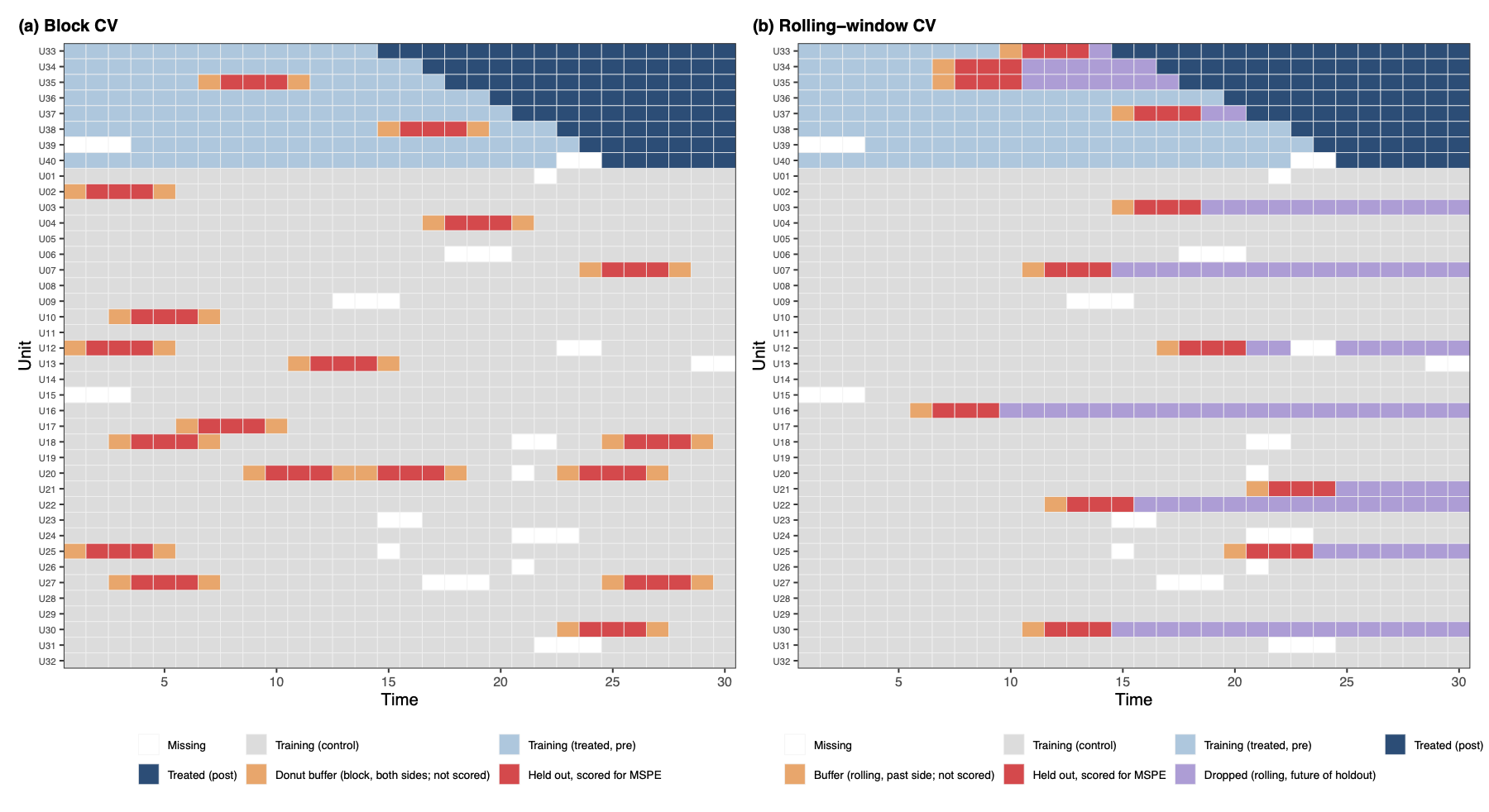
4.3.2 Rolling-window CV at a glance
Block CV (cv.method = "block") and rolling CV (cv.method = "rolling") differ in how the holdout cells are positioned within each unit’s time series. Block CV drops random scattered anchors and masks cv.nobs contiguous cells flanked on both sides by training observations, which lets serially correlated residuals leak across the train/test boundary and inflate the apparent accuracy of high-rank models. Rolling CV positions the holdout at a per-unit anchor and drops everything from the anchor onward through the unit’s end-of-eligible, so training never sees the future of the held-out block; the past side carries a small cv.buffer to attenuate same-side AR leakage. The figure below shows both designs side-by-side.
Both designs are wired into the main fect() dispatcher; switch between them by setting cv.method. The "rolling" strategy is supported for method ∈ {"ife", "gsynth", "cfe", "mc", "both"}.
For the full parameter reference (k, cv.prop, cv.nobs, cv.donut, cv.buffer, cv.rule, min.T0, seed), the scoring-criterion options, and the K=200 simulation evidence that motivates rolling as the recommended default, see the Cross-Validation section of the cheatsheet.
out.mspe <- fect(Y ~ D + X1 + X2, data = simdata, index = c("id","time"),
                 method = "ife", CV = TRUE, r = c(0, 5),
                 criterion = "mspe", se = FALSE, parallel = TRUE, cores = 16)

out.pc <- fect(Y ~ D + X1 + X2, data = simdata, index = c("id","time"),
               method = "ife", CV = TRUE, r = c(0, 5),
               criterion = "gmspe", se = FALSE, parallel = TRUE, cores = 16)
TipSelection rule
A candidate r is selected over a smaller value only if its criterion score improves by more than 1%. This prevents overfitting to marginal improvements.
4.3.3 Parallel computing
Cross-validation can be computationally expensive, especially with cv.method = "block" or "rolling" (which re-estimate the full factor or low-rank model k times per candidate tuning parameter). Parallel computing is enabled by default (parallel = TRUE); on large panels, the CV step engages multiple workers automatically.
4.3.3.1 Auto-threshold
When parallel = TRUE, parallel CV auto-activates only when the control panel is large enough that worker startup and serialization overhead are amortized by per-fold compute time. The thresholds are method-specific:
| Method | Auto-engage threshold (\(N_{co} \times T\)) | Notes |
|---|---|---|
"ife" |
20,000 | EM-based factor estimation; per-fit cost scales linearly |
"mc" |
20,000 | SVD-based; similar cost profile to IFE |
"cfe" |
60,000 | Higher per-fit overhead; smaller panels lose to serialization |
Below these thresholds, the CV runs serially even with parallel = TRUE. To force CV parallelism on a smaller panel — for example, when the per-fit time is large because \(r\) or \(k\) is high — pass parallel = "cv" (string form), which bypasses the auto-threshold and engages workers regardless of panel size.
4.3.3.2 What runs in parallel
Parallel work is organized over each (rank, fold) pair, or each (lambda, fold) pair for MC. These tasks are distributed to workers using future_lapply. This can lead to large speed gains when there are many tasks. For example, with r=c(0,5) and k=20, each CV run has 120 tasks. The "loo" method, including the older "treated_units" option, always runs sequentially because each fold depends on results computed for a given rank.
4.3.3.3 MC-specific note: early stop
For MC cross-validation in serial mode, the lambda search can stop early using the break_check rule once MSPE stops improving. In parallel mode, all candidate lambdas are evaluated because tasks are sent out at the start. As a result, when the best lambda is among the first few values, parallel mode may do more total work than serial mode. It can still be faster in wall-clock time because many folds run at once. When early stopping would apply, parallel = FALSE may be preferable.
4.3.3.4 CV vs. bootstrap, independent control
The parallel argument controls parallel computing for both CV and the bootstrap. To enable one but not the other, use parallel = "cv" or parallel = "boot". For example, during debugging, you may keep the bootstrap serial while running CV in parallel. See the parallel-computing callout in Chapter 2 for the full table.
4.4 Diagnostics
We provide three types of diagnostic tests: (1) a placebo test, (2) a joint test for (no) pretrend, and (3) a test for (no) carry-over effects. For each test, we support both the difference-in-means approach and the equivalence approach. The details are provided in the paper. We demonstrate each test using both the IFE and MC estimators.
4.4.1 Placebo tests
We provide a placebo test for a settled model—hence, cross-validation is not allowed—by setting placeboTest = TRUE. We specify a range of pre-treatment periods as “placebo periods” in option placebo.period to remove observations in the specified range for model fitting, and then test whether the estimated ATT in this range is significantly different from zero. Below, we set c(-2, 0) as the placebo periods.
We set max.iteration = 20000 to allow full convergence of the IFE model with tol = 1e-5.
out.ife.p <- fect(Y ~ D + X1 + X2, data = simdata, index = c("id", "time"),
  force = "two-way", method = "ife",  r = 2, CV = 0,
  parallel = TRUE, cores = 16, se = TRUE,
  nboots = 200, placeboTest = TRUE, placebo.period = c(-2, 0),
  max.iteration = 20000)

out.mc.p <- fect(Y ~ D + X1 + X2, data = simdata, index = c("id", "time"),
  force = "two-way", method = "mc",  lambda = out.mc$lambda.cv,
  CV = 0, parallel = TRUE, cores = 16, se = TRUE,
  nboots = 200, placeboTest = TRUE, placebo.period = c(-2, 0))
The IFE call sets max.iteration = 20000. Placebo and carryover tests drop a window of cells from the IFE estimation, which slows EM convergence below the default cap of 5000 iterations. With the smaller effective sample, EM here converges around iteration 8500. The same argument is used in the carryover and carryover.rm calls below. The MC fits do not need it, since matrix completion does not run the same EM loop.
The placebo test conducts two types of tests:
t test. If t-test p-value is smaller than a pre-specified threshold (e.g. 5%), we reject the null of no-differences. Hence, the placebo test is deemed failed.
TOST. The TOST checks whether the 90% confidence intervals for estimated ATTs in the placebo period exceed a pre-specified range (defined by a threshold), or the equivalence range. A TOST p-value smaller than a pre-specified threshold suggests that the null of difference bigger than the threshold is rejected; hence, the placebo test is passed.
By default, the plot will display the p-value of the \(t\)-test (stats = "placebo.p"). Users can also add the p-value of a corresponding TOST test by setting stats = c("placebo.p","equiv.p"). A larger placebo p-value from a t-test and a smaller placebo TOST p-value are preferred.


The placebo periods render as orange triangles on a plain panel. Pass highlight.fill = TRUE to add a lightened-tone background rectangle behind the placebo window (useful for slide / talk figures) or highlight = FALSE to suppress the accent entirely.
The results in the placebo test confirm that IFEct is a better model than MC for this particular DGP.
4.4.2 LOO pre-trend test
Instead of using estimated ATTs for periods prior to the treatment to test for pre-trends, we recommend users employ a leave-one-out (LOO) approach (loo = TRUE) to consecutively hide one pre-treatment period (relative to the timing of the treatment) and repeatedly estimate the pseudo treatment effects for that pre-treatment period. The LOO approach can be understood as an extension of the placebo test. It has the benefit of providing users with a more holistic view of whether the identifying assumptions likely hold. However, as the program needs to conduct uncertainty estimates for each turn, it is much more time-consuming than the original one.
out.ife.loo <- fect(Y ~ D + X1 + X2, data = simdata, index = c("id","time"),
  method = "ife", force = "two-way", se = TRUE, parallel = TRUE, cores = 16, nboots = 200, loo = TRUE)
out.mc.loo <- fect(Y ~ D + X1 + X2, data = simdata, index = c("id","time"),
  method = "mc", force = "two-way", se = TRUE, parallel = TRUE, cores = 16, nboots = 200, loo = TRUE)
After the LOO estimation, one can plot these LOO pre-trends in the gap plot or the equivalence plot by setting loo = TRUE in the plot function. Since all pre-treatment estimates are now out-of-sample, the plot uses a uniform black color for all points (no gray/black distinction). The equivalence plots below use the LOO estimates directly.
4.4.3 Joint tests
We now introduce two statistical tests for the presence of a pre-trend (or the lack thereof) that jointly assess pre-trend quality. The first test is an \(F\) test for zero residual averages in the pre-treatment periods. The second test is a two-one-sided \(t\) (TOST) test, a type of equivalence tests.
F test. We offer a goodness-of-fit test (a variant of the \(F\) test) and to gauge the presence of pre-treatment (differential) trends. A larger F-test p-value suggests a better pre-trend fitting. Users can specify a test range in option pre.periods. For example, pre.periods = c(-4,0) means that we test pre-treatment trend of the last 5 periods prior to the treatment (from period -4 to period 0). If pre.period = NULL (default), all pre-treatment periods in which the number of treated units exceeds the total number of treated units * proportion will be included in the test.
TOST. The TOST checks whether the 90% confidence intervals for estimated ATTs in the pre-treatment periods (again, subject to the proportion option) exceed a pre-specified range, or the equivalence range. A smaller TOST p-value suggests a better pre-trend fitting. While users can check the values of confidence intervals, we give a visualization of the equivalence test. We can plot the pre-treatment residual average with the equivalence confidence intervals by setting type = "equiv". Option tost.threshold sets the equivalence range (the default is \(0.36\sigma_{\epsilon}\) in which \(\sigma_{\epsilon}\) is the standard deviation of the outcome variable after two-way fixed effects are partialed out). By setting range = "both", both the minimum range (in gray) and the equivalence range (in red) are drawn.
On the topleft corner of the graph, we show several statistics of the user’s choice. User can choose which statistics to show by setting stats = c("none", "F.stat", "F.p", "F.equiv.p", "equiv.p") which corresponds to not showing any, the \(F\) statistic, the p-value for the \(F\) test, the p-value for the equivalence \(F\) test, the (maximum) p-value for the TOST tests, respectively. For the gap plot, the default is stats = "none". For the equivalence plot, the default is stats = c("equiv.p, F.p"). Users can also change the labels of statistics using the stats.labs options. Users can adjust its position using the stats.pos option, for example stats.pos = c(-30, 4). To turn off the statistics, set stats = "none".
Below, we visualize the result of the joint pre-trend test for each of the two estimators using our simulated data. We use the LOO estimates computed above, which provide a more honest out-of-sample pre-trend assessments.
NoteWhy LOO for pre-trend testing?
In-sample pre-trend estimates can be misleadingly close to zero because the model is fitted to these same observations. LOO provides genuine out-of-sample estimates, giving a more honest assessment of whether the parallel trends assumption holds.


From the above plots, we see that IFEct passes both tests using a conventional test size (5%); and MC fails the F tests, but passes the TOST (equivalence) test. Hence, we may conclude that IFEct is a more suitable model.
4.4.4 Carryover effects
The idea of the placebo test can be extended to testing the presence of carryover effects. Instead of hiding a few periods right before the treatment starts, we hide a few periods right after the treatment ends. If carryover effects do not exist, we would expect the average prediction error in those periods to be close to zero. To perform the carryover test, we set the option carryoverTest = TRUE. We can treat a range of exit-treatment periods in option carryover.period to remove observations in the specified range for model fitting, and then test whether the estimated ATT in this range is significantly different from zero.
Below, we set carryover.period = c(1, 3). As we deduct the treatment effect from the outcome in simdata, we expect the average prediction error for these removed periods to be close to zero.
out.ife.c <- fect(Y ~ D + X1 + X2, data = simdata, index = c("id", "time"),
  force = "two-way", method = "ife", r = 2, CV = 0,
  parallel = TRUE, cores = 16, se = TRUE,
  nboots = 200, carryoverTest = TRUE, carryover.period = c(1, 3),
  max.iteration = 20000)

out.mc.c <- fect(Y ~ D + X1 + X2, data = simdata, index = c("id", "time"),
  force = "two-way", method = "mc",  lambda = out.mc$lambda.cv,
  CV = 0, parallel = TRUE, cores = 16, se = TRUE,
  nboots = 200, carryoverTest = TRUE, carryover.period = c(1, 3))
Like the placebo test, the plot will display the p-value of the carryover effect test (stats = "carryover.p"). Users can also add the p-value of a corresponding TOST test by setting stats = c("carryover.p","equiv.p"). In exit plots, pre-exit estimates are shown in black (out-of-sample) and post-exit estimates in gray (in-sample).
plot(out.ife.c, type = "exit", main = "Carryover Effects (IFE)")

Carryover periods render as blue diamonds. As with the placebo plot, pass highlight.fill = TRUE to add a background rectangle. When several test types are active on the same fit (placebo + carryover, or carryover + carryover.rm), highlight = "carryover" (a character subset of c("placebo", "carryover", "carryover.rm")) restricts the accent treatment to a single type — the others render as plain pre/post circles.
Once again, the IFE estimator outperforms the other two.
Using real-world data, researchers will likely find that carryover effects exist. If such effects are limited, researchers can consider removing a few periods after the treatment ended for the treated units from the first-stage estimation (using the carryover.period option) and re-estimated the model (and re-conduct the test). We provide such an example in the paper. Here, we illustrate the option using simdata.
plot(out.ife.rm.test)
This fit has two test-type periods active at once:
- the three
carryover.rmperiods that were removed from the first-stage factor-model estimation, rendered as orange triangles, and - the three
carryover.periodperiods that were kept and used to test for residual carryover, rendered as blue diamonds.
The shape distinction (triangle vs diamond) holds across modern and legacy recipes, so it survives grayscale printing.
When you only need to draw attention to one of the two types, pass highlight = "carryover" or highlight = "carryover.rm"; the unselected type then renders as a plain pre/post circle:
plot(out.ife.rm.test, highlight = "carryover",
     main = "Highlight only the carryover-test periods (blue diamonds)")
plot(out.ife.rm.test, highlight = "carryover.rm",
     main = "Highlight only the removed periods (orange triangles)")
To add the lightened-tone background rectangle behind every highlight period (slide / talk style), pass highlight.fill = TRUE:
plot(out.ife.rm.test, highlight.fill = TRUE,
     main = "Both test types highlighted, with rectangles")
See Chapter 11 for the full table of highlight / highlight.fill patterns.
4.4.5 Summary
| Test | Purpose | Key arguments | Plot type | Statistics shown |
|---|---|---|---|---|
| Placebo test | Tests whether the model produces zero ATT in withheld pre-treatment periods |
placeboTest = TRUE, placebo.period = c(a, b)
|
"gap" (default) |
placebo.p, equiv.p
|
| LOO pre-trend test | Out-of-sample check for pre-trends by leaving out one pre-treatment period at a time |
loo = TRUE (in fect()), loo = TRUE (in plot()) |
"gap" or "equiv"
|
F.p, equiv.p
|
| Joint pre-trend test (F + TOST) | Joint assessment: F test for zero residual averages; TOST for equivalence within a threshold |
type = "equiv" in plot(), tost.threshold
|
"equiv" |
F.p, F.equiv.p, equiv.p
|
| Carryover test | Tests whether treatment effects persist after treatment ends |
carryoverTest = TRUE, carryover.period = c(a, b)
|
"exit" |
carryover.p, equiv.p
|
- A larger F-test / placebo / carryover p-value suggests the model passes the test.
- A smaller TOST / equivalence p-value suggests the pre-trends or carryover effects are within an acceptable range.
- We recommend using
loo = TRUEfor pre-trend tests to avoid the false reassurance of in-sample fit. - The
proportionoption controls which pre-treatment periods are included in the tests (default: periods where the number of treated units exceedsproportion\(\times\) total treated units). - The
tost.thresholdoption sets the equivalence range for the TOST test (default: \(0.36\hat{\sigma}_\epsilon\)). Finding the “right” threshold is often a challenge in empirical research.
4.5 Weights
fect() accepts a weight column via W, plus two finer-grained arguments, W.est and W.agg, that separately control whether the weight enters the outcome-model fit and whether it enters the across-treated-obs aggregation. W.est and W.agg default to NULL and fall back to W when unset, so single-column callers see the simple W-weighted behavior. For a worked example, see Chapter 2 §User-supplied weights.
-
Survey or sample weights. Pass
W = "ws". The same column applies to both the model fit and the aggregation. This is the standard treatment when the weight reflects the sampling design. -
Weight only in the outcome-model fit. Pass
W.est = "wr"alone. The weight enters the IFE / MC / CFE solver but the across-treated-obs aggregation gives each treated cell weight 1. Use this when the weight reflects fit-side considerations (e.g., a precision weight specific to the outcome model) and the estimand is the unweighted average ATT across treated cells. -
Weight only in the aggregation. Pass
W.agg = "your_column"alone. The outcome model is fit unweighted and the weight is applied only when summarizing across treated cells. Common cases include calibration weights to a target population, or post-stratification weights that should adjust the summary but not the model fit.
WarningIf your weights are inverse-probability weights for confounding adjustment
A clean in-package solution is under development for fect 3.0 (a cross-fit doubly-robust path). fect 2.3.1 does not include a recommended IPW-for-confounding workflow, and W.agg should not be used as a substitute — it does not deliver the doubly-robust properties an IPW user expects. If you need to ship analysis before v3.0 lands, see standard textbook treatments (e.g., trimming on extreme propensities) and document your design choice; we’ll point users to the in-package option once it is available.
4.6 How to Cite
If you find these methods helpful, you can cite Liu et al. (2024).
@article{LWX2024,
  title = {A Practical Guide to Counterfactual Estimators for Causal Inference with Time-Series Cross-Sectional Data},
  author = {Liu, Licheng and Wang, Ye and Xu, Yiqing},
  journal = {American Journal of Political Science},
  volume = {68},
  number = {1},
  pages = {160--176},
  year = {2024}
}