Tutorial
tutorial.RmdExample 1: Returns to Office of China’s NPC
We illustrate tjbal using a dataset from Truex (2014), in which the author investigates the returns to seats in China’s National People’s Congress by CEOs of listed firms. The dataset npc is shipped with the tjbal package (we dropped one treated firm with extremely large revenue in 2007 to improve overlap between the treated and control units; see details in the paper). To load the package and the dataset:
library(tjbal)
#> ## Syntax has changed since v.0.4.0.
#> ## See http://bit.ly/tjbal4r for more info.
#> ## Comments and suggestions -> yiqingxu@stanford.edu.
data(tjbal)
ls()
#> [1] "germany" "npc"
head(npc)
#>    gvkey fyear        roa treat so_portion  rev2007
#> 1 108893  2005 0.13556981     0  0.5286272 15110.46
#> 2 108893  2006 0.10115566     0  0.5286272 15110.46
#> 3 108893  2007 0.12335894     0  0.5286272 15110.46
#> 4 108893  2008 0.20065501     1  0.5286272 15110.46
#> 5 108893  2009 0.06594828     1  0.5286272 15110.46
#> 6 108893  2010 0.12756890     1  0.5286272 15110.46
First, we take a look at the data structure. The outcome variable is
roa and the treatment indicator is treat; the
unit and time indicators are gvkey and fyear,
respectively. There are 47 treated firms whose CEOs became NPC members
in 2008 and 939 control firms whose CEOs were never NPC members from
2005 to 2010.
The following plot shows the treatment status of the first 50 firms based on firm ID:
library(panelView)
#> ## See bit.ly/panelview4r for more info.
#> ## Report bugs -> yiqingxu@stanford.edu.
panelview(roa ~ treat + so_portion + rev2007, data = npc, show.id = c(1:50),
          index = c("gvkey","fyear"), xlab = "Year", ylab = "Firm ID",
          axis.lab.gap = c(0,1), by.timing = TRUE,
          display.all = TRUE, axis.lab = "time")
#> If the number of units is more than 300, we set "gridOff = TRUE".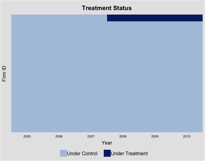
with(npc, table(fyear, treat))
#>       treat
#> fyear    0   1
#>   2005 986   0
#>   2006 986   0
#>   2007 986   0
#>   2008 939  47
#>   2009 939  47
#>   2010 939  47
Difference-in-Differences (DID)
We then apply the difference-in-differences (DiD) method without
controlling for any covariates. In the formula of
tjbal, the left-hand-side variable is the outcome and
the first right-hand-side variable is the dichotomous treatment
indicator. We specify unit and time indicators using the
index option. At the moment, we do not want to balance on
pre-treatment outcomes, therefore, we set Y.match.npre = 0.
Because an DID approach involves subtracting pre-treatment means from
the outcome for each unit, we set demean = TRUE.
Uncertainty estimates are obtained via a bootstrap procedure.
tjbal provides three balancing approaches: (1)
"mean", which stands for mean-balancing; (2)
"kernel", which stands for kernel-balancing; and (3)
"meanfirst", which stands for kernel balancing with mean
balancing constraints. "meanfirst" will prioritize
balancing on covariate means over higher-order terms and interactions.
The default option is "meanfirst". In this case, because we
do not have any covariates to seek balance on, the
estimator option is redundant.
For datasets with only one treatment timing, tjbal
provides three types of uncertainty estimates:
vce = "fixed.weights" which treats balancing weights as
fixed; "jackknife" (or "jack"), which conducts
jackknife by omitting one treated unit at a time, and
"bootstrap" (or "boot"), which conducts
non-parametric bootstrapping by reshuffle both the treated and control
units. We show in the paper that, with reasonably large samples, these
three methods yield very similar results. When "jackknife"
or "bootstrap" is chosen, nsims determines the
number of jackknife or bootstrap runs. With jackknife,
nsims will be ignored if it is bigger than the number of
treated units.
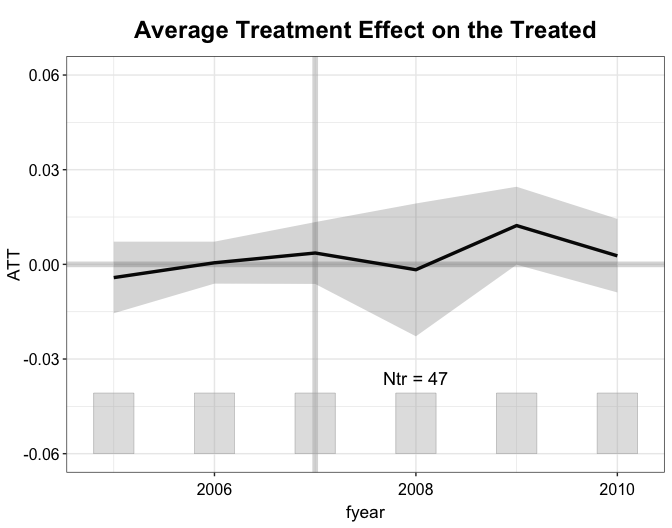
The print function present the result, which shows a non-significant effect of NPC membership on firms’ return on assets (ROA).
out.did <- tjbal(roa ~ treat, data = npc,
index = c("gvkey","fyear"), Y.match.npre = 0,
demean = TRUE, vce = "boot", nsims = 200)
#>
#> Bootstrapping...
#> Parallel computing...
print(out.did)
#> Call:
#> tjbal.formula(formula = roa ~ treat, data = npc, index = c("gvkey",
#> "fyear"), Y.match.npre = 0, demean = TRUE, vce = "boot",
#> nsims = 200)
#>
#> ~ by Period (including Pre-treatment Periods):
#> ATT S.E. z-score CI.lower CI.upper p.value n.Treated
#> 2005 -0.0042 0.0061 -0.6851 -0.0160 0.0077 0.4933 47
#> 2006 0.0005 0.0038 0.1428 -0.0069 0.0080 0.8865 47
#> 2007 0.0036 0.0047 0.7620 -0.0057 0.0129 0.4461 47
#> 2008 -0.0017 0.0106 -0.1644 -0.0225 0.0190 0.8694 47
#> 2009 0.0123 0.0068 1.8186 -0.0010 0.0255 0.0690 47
#> 2010 0.0027 0.0062 0.4437 -0.0094 0.0149 0.6573 47
#>
#> Average Treatment Effect on the Treated:
#> ATT S.E. z-score CI.lower CI.upper p.value
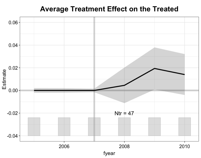
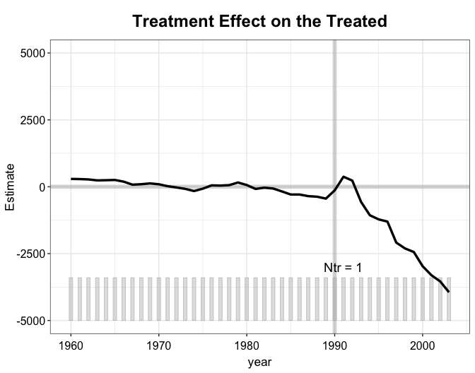
#> [1,] 0.0044 0.0063 0.706 -0.0079 0.0167 0.4802The plot function visualizes the result, By default
(type = gap), it plots the average treatment effect on the
treated (ATT) over time (from 2008 to 2010). We add a histogram to
illustrate the number of treated units at the bottom of the figure. It
can be turned off by setting count == FALSE.
We can also plot the treated and estimated \(Y(0)\) averages by specifying
type = "counterfactual or simply type = "ct".
Note that, with the DID approach, the estimated \(Y(0)\) averages do not fit perfectly with
the treated averaged over the pre-treatment periods.
plot(out.did, type = "counterfactual", count = FALSE)
The plot function can also visualize the distribution of weights of the control units (the total weights added up to \(N_{tr}\), the number of the treated units). With the DID method, all control units are equally weighted:
plot(out.did, type = "weights")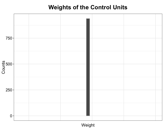
Mean Balancing
Next, we apply the mean balancing approach (which the author uses in
the original paper). In the formula, we also add two covariates,
so_portion and rev2007. Note that they will
not be put into regressions directly; rather, the algorithm will seek
balance on them as well as the three pre-treatment outcomes. Because we
do not employ the kernel transformation, we set
estimator = "mean".
out.mbal <- tjbal(roa ~ treat + so_portion + rev2007, data = npc,
index = c("gvkey","fyear"), demean = FALSE, estimator = "mean",
vce = "jackknife")
#> Seek balance on:
#> roa2005, roa2006, roa2007, so_portion, rev2007
#>
#> Optimization:
#> bias.ratio = 0.0000; num.dims = 5 (mbal)
#>
#> Balance Table
#> mean.tr mean.co.pre mean.co.pst sd.tr sd.co.pre sd.co.pst
#> roa2005 0.0376 0.0225 0.0376 0.0675 0.0801 0.0778
#> roa2006 0.0503 0.0305 0.0503 0.0424 0.0756 0.0667
#> roa2007 0.0643 0.0414 0.0643 0.0564 0.1035 0.1611
#> so_portion 0.3170 0.2491 0.3170 0.2397 0.2218 0.2355
#> rev2007 6420.3705 2647.3412 6420.3705 9547.6633 5530.8308 14355.1192
#> diff.pre diff.pst
#> roa2005 0.2243 0
#> roa2006 0.4682 0
#> roa2007 0.4062 0
#> so_portion 0.2835 0
#> rev2007 0.3952 0
#>
#> Jackknife...
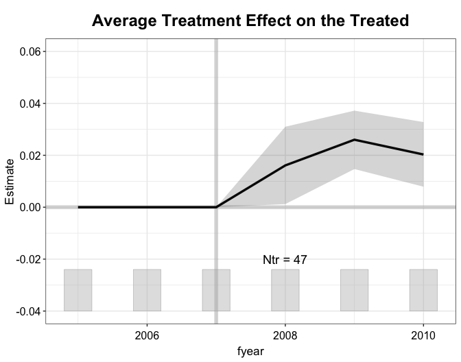
#> Parallel computing...We see that NPC membership increases ROA by about 2 percentage points, and it is highly statistically significant.
print(out.mbal)
#> Call:
#> tjbal.formula(formula = roa ~ treat + so_portion + rev2007, data = npc,
#>     index = c("gvkey", "fyear"), demean = FALSE, estimator = "mean",
#>     vce = "jackknife")
#>
#>    ~ by Period (including Pre-treatment Periods):
#>         ATT   S.E. z-score CI.lower CI.upper p.value n.Treated
#> 2005 0.0000 0.0000  0.0001   0.0000   0.0000  0.9999        47
#> 2006 0.0000 0.0000 -0.0038   0.0000   0.0000  0.9969        47
#> 2007 0.0000 0.0000 -0.0054   0.0000   0.0000  0.9957        47
#> 2008 0.0161 0.0076  2.1216   0.0012   0.0310  0.0339        47
#> 2009 0.0260 0.0057  4.5312   0.0147   0.0372  0.0000        47
#> 2010 0.0203 0.0064  3.1939   0.0079   0.0328  0.0014        47
#>
#> Average Treatment Effect on the Treated:
#>         ATT   S.E. z-score CI.lower CI.upper p.value
#> [1,] 0.0208 0.0057   3.628   0.0096    0.032   3e-04
Alternatively, we can also specify the outcome (Y),
treatment (D), and covariates (X)
separately.
out.mbal <- tjbal(data = npc, Y = "roa", D = "treat", X = c("so_portion","rev2007"),
  index = c("gvkey","fyear"), demean = FALSE, estimator = "mean",
  vce = "jackknife", nsims = 200)
We show the gap plot, the counterfactual
plot, and the weightsplot again. With mean balancing, the
pre-treatment outcomes are perfectly balanced between the treatment and
control groups.
plot(out.mbal, type = "ct")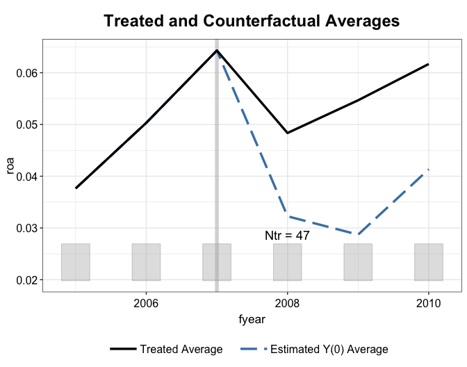
We can also add two bands that represent the ranges of the 5 to 95%
quantile of the treated and control trajectories to the plot by setting
raw = "band". When trim = TRUE (default), the
control group data will be trimmed based on weights assigned to the
control units (up to 90% of the total weight).
We can change the font size of almost all elements in the figure by
setting cex.main (for title), cex.lab (for
axis titles), cex.axis (for numbers on the axes),
cex.legend (for legend) and cex.text for text
in the figure. The numbers are all relative to the default.
A set of legend options can be used to adjust the look of the
legends, including legendOff (turn off legends),
legend.pos (position), legend.ncol (number of
columns), and legend.labs (change label texts).
plot(out.mbal, type = "ct", raw = "band", ylim = c(-0.2, 0.3),
     cex.main = 0.9, cex.lab = 1.1, cex.axis = 0.9, cex.legend= 0.8, cex.text = 1.5,
     legend.pos = "top")
plot(out.mbal, type = "weights")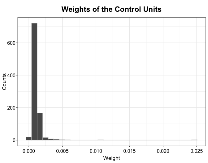
The plot function can also check balance in pre-treatment outcomes and covariates between the treatment and control groups before and after reweighting:
plot(out.mbal, type = "balance")
Kernel Balancing (w/ mean balancing constraints)
Finally, we apply the kernel balancing method (while respecting
mean-balancing constraints) by setting
estimator = "meanfirst". Note that kernel balancing is
significantly more computationally intensive than mean balancing.
Parallel computing with 4 cores on a 2016 iMac takes about 1 minutes to
finish 47 jackknife runs.
begin.time<-Sys.time()
out.kbal <- tjbal(roa ~ treat + so_portion + rev2007, data = npc,
  index = c("gvkey","fyear"), estimator = "meanfirst", demean = FALSE, vce = "jackknife")
#> Seek balance on:
#> roa2005, roa2006, roa2007, so_portion, rev2007
#>
#> Optimization:
#> bias.ratio = 0.0950; num.dims = 5 + 43 (mbal + kbal)
#>
#> Balance Table
#>              mean.tr mean.co.pre mean.co.pst     sd.tr sd.co.pre sd.co.pst
#> roa2005       0.0376      0.0225      0.0376    0.0675    0.0801    0.0658
#> roa2006       0.0503      0.0305      0.0503    0.0424    0.0756    0.0425
#> roa2007       0.0643      0.0414      0.0643    0.0564    0.1035    0.0541
#> so_portion    0.3170      0.2491      0.3170    0.2397    0.2218    0.2378
#> rev2007    6420.3705   2647.3412   6420.3704 9547.6633 5530.8308 9410.3702
#>            diff.pre diff.pst
#> roa2005      0.2243        0
#> roa2006      0.4682        0
#> roa2007      0.4062        0
#> so_portion   0.2835        0
#> rev2007      0.3952        0
#>
#> Jackknife...
#> Parallel computing...
print(Sys.time()-begin.time)
#> Time difference of 1.50954 mins
With kernel balancing with mean balancing weights, we find that NPC membership of the CEO increases a firm’s ROA by 1.4 percentage points. The estimate remains highly statistically significant.
print(out.kbal)
#> Call:
#> tjbal.formula(formula = roa ~ treat + so_portion + rev2007, data = npc,
#>     index = c("gvkey", "fyear"), demean = FALSE, estimator = "meanfirst",
#>     vce = "jackknife")
#>
#>    ~ by Period (including Pre-treatment Periods):
#>         ATT   S.E. z-score CI.lower CI.upper p.value n.Treated
#> 2005 0.0000 0.0011  0.0000  -0.0021   0.0021  1.0000        47
#> 2006 0.0000 0.0010  0.0000  -0.0020   0.0020  1.0000        47
#> 2007 0.0000 0.0008  0.0000  -0.0016   0.0016  1.0000        47
#> 2008 0.0045 0.0080  0.5665  -0.0112   0.0202  0.5711        47
#> 2009 0.0194 0.0095  2.0469   0.0008   0.0380  0.0407        47
#> 2010 0.0140 0.0092  1.5231  -0.0040   0.0321  0.1277        47
#>
#> Average Treatment Effect on the Treated:
#>         ATT   S.E. z-score CI.lower CI.upper p.value
#> [1,] 0.0127 0.0068   1.851   -7e-04   0.0261  0.0642
Balance (in means) in the pre-treatment outcomes and covariates remain great, but no longer perfect. This is because kernel balancing also attempts to achieve balance in high-order features of these variables.
plot(out.kbal, type = "ct", xlab = "Year", ylab = "Return to Assets")
plot(out.kbal, type = "weights")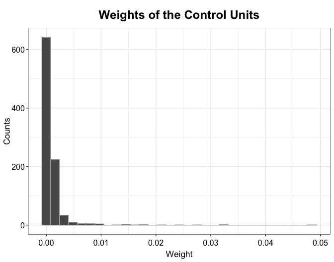
plot(out.kbal, type = "balance")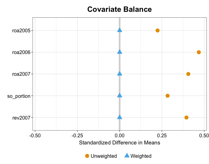
For example, kernel balancing also makes the standard deviations (or variance) of these variables in the treatment and reweighted control groups more similar than mean balancing.
plot(out.mbal, type = "balance", stat = "sd")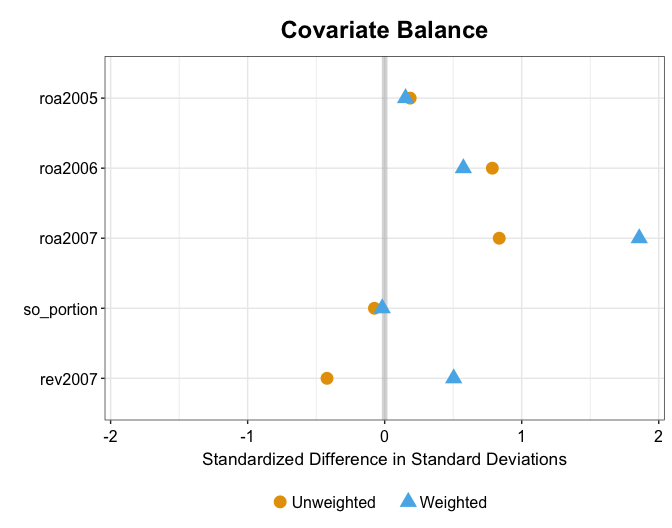
plot(out.kbal, type = "balance", stat = "sd")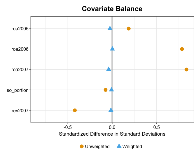
For this example, setting estimator = "kernel"
(i.e. kernel balancing without incorporating mean balancing constraints)
yields very similar results.
Example 2: German Reunification
In the second example, we re-investigate the effect of German
reunification on West Germany’s GDP growth using data from Abadie, Diamond, and Hainmueller (2015).
Variable treat indicate West Germany over the post-1990
periods. Again, we look at the data structure first:
panelview(data = germany, gdp ~ treat, index = c("country","year"),
          xlab = "Year", ylab = "Country", by.timing = TRUE,
          axis.adjust = TRUE, axis.lab.gap = c(1,0))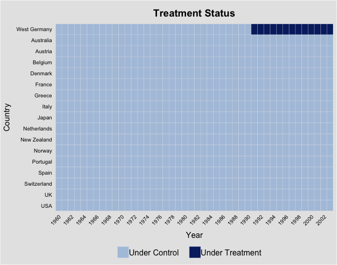
Next, we implement the mean balancing method. Different from the
previous example, we take averages for the covariates over different
time periods (to be consistent with the original paper). Make sure that
the length of the list set by X.avg.time is the the same as
the length of the variable names in X.
out2.mbal <- tjbal(data = germany, Y = "gdp", D = "treat", Y.match.time = c(1960:1990),
  X = c("trade","infrate","industry", "schooling", "invest80"),
  X.avg.time = list(c(1981:1990),c(1981:1990),c(1981:1990),c(1980:1985),c(1980)),
  index = c("country","year"), demean = TRUE)
#> Too few treated unit(s). Uncertainty estimates not provided.
#> Seek balance on:
#> gdp.dm1960, gdp.dm1961, gdp.dm1962, gdp.dm1963, gdp.dm1964, gdp.dm1965, gdp.dm1966, gdp.dm1967, gdp.dm1968, gdp.dm1969, gdp.dm1970, gdp.dm1971, gdp.dm1972, gdp.dm1973, gdp.dm1974, gdp.dm1975, gdp.dm1976, gdp.dm1977, gdp.dm1978, gdp.dm1979, gdp.dm1980, gdp.dm1981, gdp.dm1982, gdp.dm1983, gdp.dm1984, gdp.dm1985, gdp.dm1986, gdp.dm1987, gdp.dm1988, gdp.dm1989, gdp.dm1990, trade, infrate, industry, schooling, invest80
#>
#> Optimization:
#> bias.ratio = 0.5468; num.dims = 2 + 0 (mbal + kbal)
#>
#> Balance Table
#>               mean.tr mean.co.pre mean.co.pst diff.pre diff.pst
#> gdp.dm1960 -6282.4516  -5549.6673  -6575.8498  -0.1166   0.0467
#> gdp.dm1961 -6178.4516  -5438.3548  -6465.1921  -0.1198   0.0464
#> gdp.dm1962 -6039.4516  -5319.6673  -6313.2363  -0.1192   0.0453
#> gdp.dm1963 -5956.4516  -5207.3548  -6194.2952  -0.1258   0.0399
#> gdp.dm1964 -5760.4516  -5053.4798  -6005.0548  -0.1227   0.0425
#> gdp.dm1965 -5561.4516  -4901.0423  -5815.6146  -0.1187   0.0457
#> gdp.dm1966 -5398.4516  -4711.6673  -5589.3747  -0.1272   0.0354
#> gdp.dm1967 -5325.4516  -4556.1048  -5402.9393  -0.1445   0.0146
#> gdp.dm1968 -4995.4516  -4292.0423  -5090.7819  -0.1408   0.0191
#> gdp.dm1969 -4568.4516  -3937.3548  -4693.9368  -0.1381   0.0275
#> gdp.dm1970 -4199.4516  -3600.3548  -4292.2593  -0.1427   0.0221
#> gdp.dm1971 -3880.4516  -3286.1673  -3901.6583  -0.1531   0.0055
#> gdp.dm1972 -3511.4516  -2929.7298  -3485.5438  -0.1657  -0.0074
#> gdp.dm1973 -3013.4516  -2434.9798  -2934.4072  -0.1920  -0.0262
#> gdp.dm1974 -2492.4516  -1929.8548  -2332.1177  -0.2257  -0.0643
#> gdp.dm1975 -1963.4516  -1482.7923  -1892.0915  -0.2448  -0.0363
#> gdp.dm1976 -1199.4516   -921.0423  -1251.1953  -0.2321   0.0431
#> gdp.dm1977  -476.4516   -381.5423   -520.8741  -0.1992   0.0932
#> gdp.dm1978   361.5484    289.7702    301.2427   0.1985   0.1668
#> gdp.dm1979  1500.5484   1157.7702   1341.5094   0.2284   0.1060
#> gdp.dm1980  2516.5484   2083.5202   2452.4602   0.1721   0.0255
#> gdp.dm1981  3548.5484   3020.6452   3629.7422   0.1488  -0.0229
#> gdp.dm1982  4194.5484   3664.8327   4228.9958   0.1263  -0.0082
#> gdp.dm1983  4952.5484   4284.3327   5018.3650   0.1349  -0.0133
#> gdp.dm1984  5914.5484   5052.1452   6089.4276   0.1458  -0.0296
#> gdp.dm1985  6724.5484   5795.8327   7014.5704   0.1381  -0.0431
#> gdp.dm1986  7431.5484   6408.8952   7721.2870   0.1376  -0.0390
#> gdp.dm1987  8112.5484   7075.5202   8463.7659   0.1278  -0.0433
#> gdp.dm1988  9219.5484   8033.7702   9592.0343   0.1286  -0.0404
#> gdp.dm1989 10427.5484   9064.5827  10870.3999   0.1307  -0.0425
#> gdp.dm1990 11898.5484  10001.5827  12032.6221   0.1594  -0.0113
#> trade         56.7778     59.8313     59.1378  -0.0538  -0.0416
#> infrate        2.5948      7.6166      4.6865  -1.9353  -0.8061
#> industry      34.5385     33.7944     32.1820   0.0215   0.0682
#> schooling     55.5000     38.6594     50.8456   0.3034   0.0839
#> invest80      27.0180     25.8952     25.5263   0.0416   0.0552
Alternatively, we can use the following syntax:
out2.kbal <- tjbal(gdp ~ treat + trade + infrate + industry + schooling + invest80,
                  data = germany, Y.match.time = c(1960:1990), X.avg.time = list(c(1981:1990), c(1981:1990), c(1981:1990),c(1980:1985),c(1980)),
                  index = c("country","year"), estimator = "kernel", demean = TRUE)
#> Too few treated unit(s). Uncertainty estimates not provided.
#> Seek balance on:
#> gdp.dm1960, gdp.dm1961, gdp.dm1962, gdp.dm1963, gdp.dm1964, gdp.dm1965, gdp.dm1966, gdp.dm1967, gdp.dm1968, gdp.dm1969, gdp.dm1970, gdp.dm1971, gdp.dm1972, gdp.dm1973, gdp.dm1974, gdp.dm1975, gdp.dm1976, gdp.dm1977, gdp.dm1978, gdp.dm1979, gdp.dm1980, gdp.dm1981, gdp.dm1982, gdp.dm1983, gdp.dm1984, gdp.dm1985, gdp.dm1986, gdp.dm1987, gdp.dm1988, gdp.dm1989, gdp.dm1990, trade, infrate, industry, schooling, invest80
#>
#> Optimization:
#> bias.ratio = 0.8091; num.dims = 1 (kbal)
#>
#> Balance Table
#>               mean.tr mean.co.pre mean.co.pst diff.pre diff.pst
#> gdp.dm1960 -6282.4516  -5549.6673  -5795.5598  -0.1166  -0.0775
#> gdp.dm1961 -6178.4516  -5438.3548  -5705.1750  -0.1198  -0.0766
#> gdp.dm1962 -6039.4516  -5319.6673  -5568.4468  -0.1192  -0.0780
#> gdp.dm1963 -5956.4516  -5207.3548  -5457.5674  -0.1258  -0.0838
#> gdp.dm1964 -5760.4516  -5053.4798  -5300.1505  -0.1227  -0.0799
#> gdp.dm1965 -5561.4516  -4901.0423  -5160.3940  -0.1187  -0.0721
#> gdp.dm1966 -5398.4516  -4711.6673  -4961.5077  -0.1272  -0.0809
#> gdp.dm1967 -5325.4516  -4556.1048  -4780.8164  -0.1445  -0.1023
#> gdp.dm1968 -4995.4516  -4292.0423  -4498.4115  -0.1408  -0.0995
#> gdp.dm1969 -4568.4516  -3937.3548  -4129.7337  -0.1381  -0.0960
#> gdp.dm1970 -4199.4516  -3600.3548  -3786.3056  -0.1427  -0.0984
#> gdp.dm1971 -3880.4516  -3286.1673  -3487.6178  -0.1531  -0.1012
#> gdp.dm1972 -3511.4516  -2929.7298  -3145.7532  -0.1657  -0.1041
#> gdp.dm1973 -3013.4516  -2434.9798  -2653.5151  -0.1920  -0.1194
#> gdp.dm1974 -2492.4516  -1929.8548  -2097.7868  -0.2257  -0.1583
#> gdp.dm1975 -1963.4516  -1482.7923  -1599.2937  -0.2448  -0.1855
#> gdp.dm1976 -1199.4516   -921.0423   -985.3133  -0.2321  -0.1785
#> gdp.dm1977  -476.4516   -381.5423   -428.6132  -0.1992  -0.1004
#> gdp.dm1978   361.5484    289.7702    275.6705   0.1985   0.2375
#> gdp.dm1979  1500.5484   1157.7702   1229.2199   0.2284   0.1808
#> gdp.dm1980  2516.5484   2083.5202   2216.4550   0.1721   0.1192
#> gdp.dm1981  3548.5484   3020.6452   3212.5685   0.1488   0.0947
#> gdp.dm1982  4194.5484   3664.8327   3897.7849   0.1263   0.0707
#> gdp.dm1983  4952.5484   4284.3327   4578.8684   0.1349   0.0755
#> gdp.dm1984  5914.5484   5052.1452   5349.6508   0.1458   0.0955
#> gdp.dm1985  6724.5484   5795.8327   6129.5811   0.1381   0.0885
#> gdp.dm1986  7431.5484   6408.8952   6766.7423   0.1376   0.0895
#> gdp.dm1987  8112.5484   7075.5202   7479.4055   0.1278   0.0780
#> gdp.dm1988  9219.5484   8033.7702   8476.1354   0.1286   0.0806
#> gdp.dm1989 10427.5484   9064.5827   9496.5271   0.1307   0.0893
#> gdp.dm1990 11898.5484  10001.5827  10433.3520   0.1594   0.1231
#> trade         56.7778     59.8313     59.2553  -0.0538  -0.0436
#> infrate        2.5948      7.6166      6.3965  -1.9353  -1.4651
#> industry      34.5385     33.7944     33.8506   0.0215   0.0199
#> schooling     55.5000     38.6594     41.2716   0.3034   0.2564
#> invest80      27.0180     25.8952     26.4878   0.0416   0.0196
We plot the estimated treatment effect from both mean balancing and kernel balancing. It seems that the kernel balancing approach yield slightly better pre-treatment fit—this is not always the case.

The estimated counterfactual for West Germany.
plot(out2.mbal, type = "counterfactual", count = FALSE) 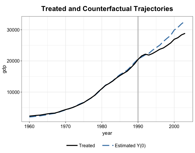
plot(out2.kbal, type = "ct", count = FALSE) 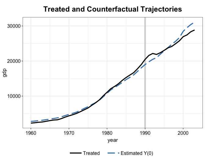
By setting raw = "all" and trim = TRUE
(default), we can add to the counterfactual plot the trajectories of the
heavily weighted control units, whose assigned weights add up to 90% of
the total weight. The number 90% can be adjusted by the
trim.wtot option. If trim = FALSE, all control
trajectories will be shown.
plot(out2.mbal, type = "ct", raw = "all", trim.wtot = 0.9) 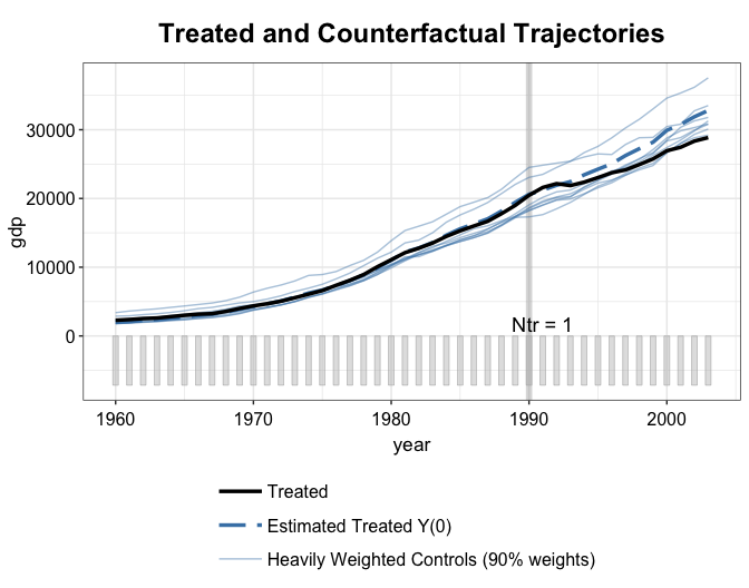
We can see that kernel balancing put more weights on a much smaller number of control units.
plot(out2.kbal, type = "ct", raw = "all") 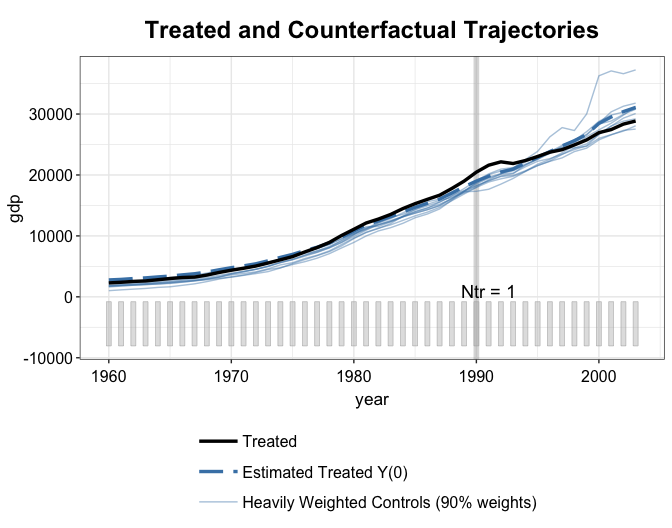
By setting raw = "band" and trim = "TRUE"
(default), we show the range of the trajectories of heavily weighted
controls.
plot(out2.mbal, type = "ct", raw = "band") 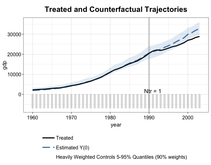
Finally, the weights plot confirms that kernel balancing
puts more weights on fewer control units.
plot(out2.mbal, type = "weights")
plot(out2.kbal, type = "weights")