Tutorial
tutorial.RmdThis page demonstrates the usage of the hbal package, which implements hierarchically regularized entropy balancing introduced by Xu and Yang (2022). hbal automatically expands the covariate space to include higher order terms and uses cross-validation to select variable penalties for the balancing conditions, and then seeks approximate balance on the expanded covariate space.
hbal provides two main functions:
hbal(): performs hierarchically regularized entropy balancing.att(): calculates the average treatment effect on the treated (ATT) from anhbalobject returned byhbal().
And two S3 methods:
summary(): summarizes the balancing results.plot(): visualizes covariate balance before and after weighting or the distribution of balancing weights.
R code used in this tutorial can be downloaded from here.
Basic Usage
We simulate a toy cross-sectional dataset with a binary treatment to illustrate the basic usage of hbal. Note that treatment assignment depends on all three covariates.
library(hbal)
set.seed(1984)
N <- 1500
X1 <- rnorm(N)
X2 <- rnorm(N)
X3 <- rbinom(N, size = 1, prob = .5)
D_star <- 0.5 * X1 + 0.3 * X2 + 0.2 * X1 * X2 - 0.5 * X1 * X3 - 1
D <- ifelse(D_star > rnorm(N), 1, 0) # Treatment indicator
y <- 0.5 * D + X1 + X2 + X2 * X3 + rnorm(N) # Outcome
dat <- data.frame(D = D, X1 = X1, X2 = X2, X3 = X3, Y = y)
head(dat)
#>   D         X1          X2 X3          Y
#> 1 0  0.4092032  1.37178450  0  0.6358481
#> 2 1 -0.3230250  0.62887225  0  1.5377304
#> 3 0  0.6358523  1.49692496  1  1.5998765
#> 4 0 -1.8461288  0.19218026  1 -1.8232558
#> 5 0  0.9536474  0.16077270  0  3.2611010
#> 6 0  1.1884898 -0.07989461  1  1.0611114
hbal is an extension of entropy balancing, or
ebal proposed by Hainmueller
(2012). By default, hbal replicates
ebal by performing exact balancing on all covariates
and no serial expansion, i.e., expand.degree = 1 (default).
We can demonstrate this equivalence by showing the hbal weights are
exactly the same to the ebal weights from the ebal
package in this case.
library(ebal)
ebal.out <- ebalance(Treat = dat$D, X = dat[,c('X1', 'X2', 'X3')]) # ebal
#> Converged within tolerance
hbal.out <- hbal(Treat = 'D', X = c('X1', 'X2', 'X3'),  Y = 'Y',  data = dat) # hbal

# plot weights
W <- data.frame(x = ebal.out$w, y = hbal.out$weights.co)
ggplot(aes(x = x, y = y), data = W) + geom_point() + theme_bw() +
  labs(x = "ebal weights", y="hbal weights", title = "ebal weights vs. hbal weights")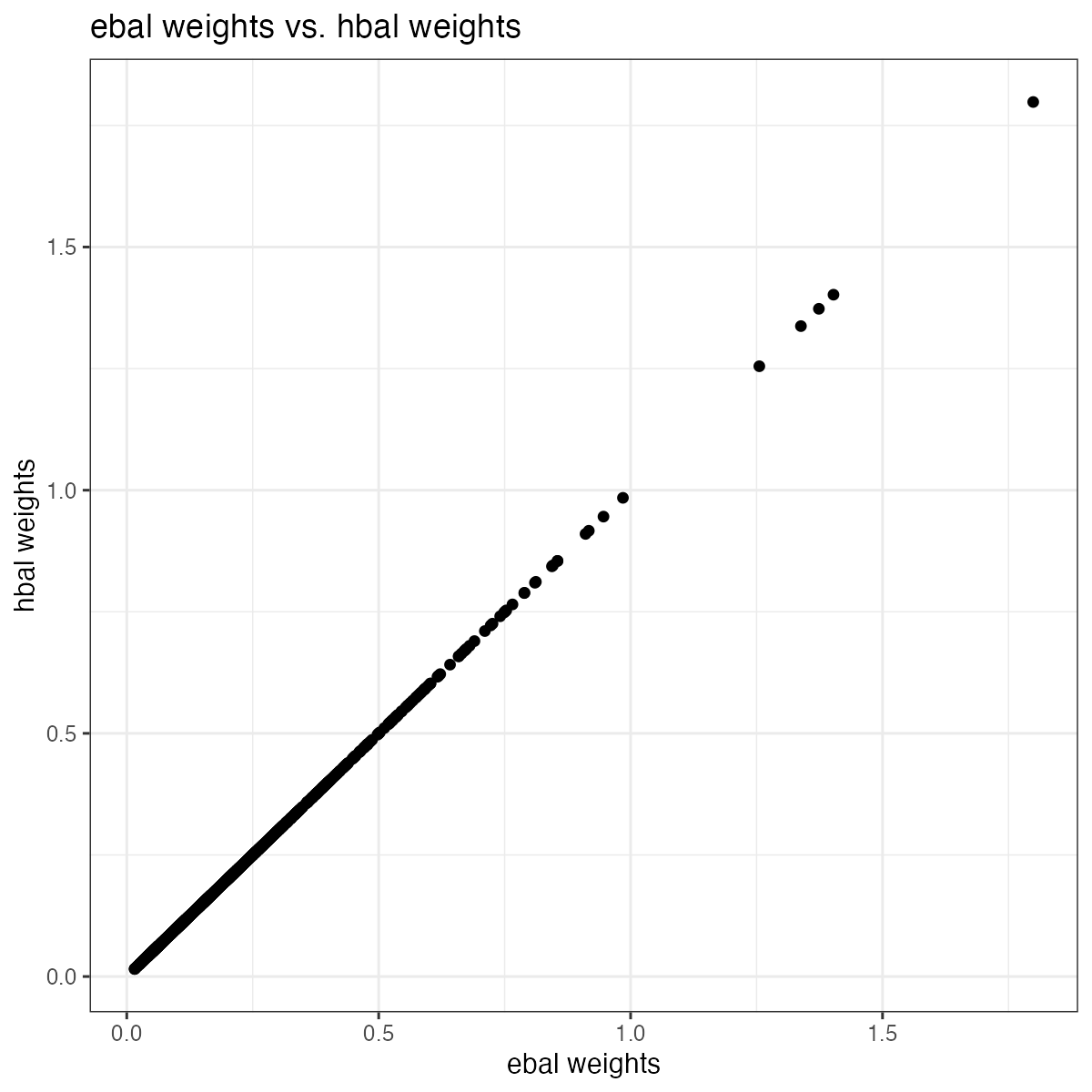
hbal() returns a list of 15 objects:
names(hbal.out)
#>  [1] "converged"     "weights"       "weights.co"    "coefs"
#>  [5] "Treatment"     "mat"           "grouping"      "group.penalty"
#>  [9] "term.penalty"  "bal.tab"       "base.weights"  "Treat"
#> [13] "Outcome" "Y" "call"- converged: Binary indicator of whether the algorithm has converged.
- weights: Resulting weights, including the base weights for the treated and solution weights for the controls (see below).
- weights.co: Solution weights for the controls. Can be plugged into any downstream estimator.
-
coefs: Values of Lagrangian multipliers. They are
used to calculate the solution
weights. - Treatment: The treatment status vector.
- mat: Data matrix, including the outcome variable (the first column), the treatment variable (the second column), and expanded covariates (the remaining columns).
- grouping: A vector of the number of variables in each covariate group. The length of the vector equals the number of groups.
- group.penalty: Penalties for different groups of covariates. This is the regularization parameter \(\alpha\) in Xu and Yang (2022).
- term.penalty: Penalties for individual covariates. The length of the vector equals the number of balancing terms, including expanded ones.
- bal.tal: A balance table.
-
base.weights: A vector of base weights, originally
from variable
wsupplied by users. The length of the vector equals the number of rows entering the balancing scheme. - Treat: A character string that stores the treatment variable name.
-
Outcome: The outcome vector, if
Yis supplied. -
Y: A character string that stores the outcome
variable name, if
Yis supplied.. - call: A string of the function call.
The summary() function provides additional information
on the balancing scheme, including the numbers of treated and control
units, groups and corresponding penalties, and a balance table, in which
Std.Diff.(O) and Std.Diff.(W) represent
standardized difference before and after balancing, respectively. For
example, in this case, only the linear terms are being balanced on.
summary(hbal.out)
#> Call:
#>  hbal(data = dat, Treat = "D", X = c("X1", "X2", "X3"), Y = "Y")
#>
#>  Treated Controls
#>      256     1244
#>  Co/Tr Ratio = 4.86
#>
#>  Groups
#>        #Terms Penalty
#> linear      3       0
#>
#>  Balance Table
#>    Tr.Mean Co.Mean W.Co.Mean Std.Diff.(O) Std.Diff.(W)
#> X1    0.35   -0.11      0.35         0.46            0
#> X2    0.42   -0.07      0.42         0.49            0
#> X3    0.52    0.51      0.52         0.02            0
In addition to balancing on just the linear/level terms of the
covariates, hbal() allows balancing on a serial expansion
of the covariates. This is achieved by setting the
expand.degree argument. Currently, hbal()
supports both second order serial expansion (two-way interactions and
square terms; expand.degree = 2) and third order serial
expansion (two-way interactions, square terms, linear*square
interactions, and cubic terms; expand.degree = 3). For
example, we can do exact balancing on third order serial expansion of
the covariates:
out <- hbal(Y = 'Y', Treat = 'D', X = c('X1', 'X2', 'X3'),
            data = dat, expand.degree = 3)
summary(out)
#> Call:
#>  hbal(data = dat, Treat = "D", X = c("X1", "X2", "X3"), Y = "Y",
#>     expand.degree = 3)
#>
#>  Treated Controls
#>      256     1244
#>  Co/Tr Ratio = 4.86
#>
#>  Groups
#>                #Terms Penalty
#> linear              3       0
#> two-way             3       0
#> squared             2       0
#> three-way           1       0
#> squared*linear      4       0
#> cubic               2       0
#>
#>  Balance Table
#>          Tr.Mean Co.Mean W.Co.Mean Std.Diff.(O) Std.Diff.(W)
#> X1          0.35   -0.11      0.35         0.46            0
#> X2          0.42   -0.07      0.42         0.49            0
#> X3          0.52    0.51      0.52         0.02            0
#> X1.X2       0.24   -0.10      0.24         0.32            0
#> X1.X3       0.07   -0.02      0.07         0.12            0
#> X2.X3       0.21   -0.01      0.21         0.33            0
#> X1.X1       1.01    1.01      1.01         0.00            0
#> X2.X2       0.99    0.99      0.99         0.00            0
#> X1.X2.X3    0.13    0.00      0.13         0.18            0
#> X1.X1.X2    0.32   -0.01      0.32         0.18            0
#> X1.X2.X2    0.32   -0.17      0.32         0.29            0
#> X1.X1.X3    0.55    0.52      0.55         0.03            0
#> X2.X2.X3    0.50    0.47      0.50         0.02            0
#> X1.X1.X1    0.93   -0.25      0.93         0.30            0
#> X2.X2.X2    1.16   -0.23      1.16         0.40            0
Obtaining the ATT
We can use att() on a hbal object to
directly get an ATT estimate. Note that att() uses linear
regression with robust standard errors (lm_robust() from
the estimatr package) to calculate the ATT.
att() allows users to use one of the following three
methods to estimate the ATT:
difference in weighted means by setting
dr = FASLE, in whichdrrepresents doubly robust; as a result,methodis ignored;weighted linear regression by setting
method = ""lm_robust"(default);weighted linear regression with a full set of interactions between the treatment indicator and demeaned covariates, or Lin’s method, by setting
method = ""lm_lin".
By default, att() only displays treatment
effect(displayAll = FALSE). Additional arguments accepted
by lm_robust() or lm_lin(), such as
se_type and clusters, can be passed to
att(), for example:
att(out, dr = FALSE)
#>    Estimate Std. Error  t value    Pr(>|t|)  CI Lower  CI Upper   DF
#> D 0.4762995  0.1598373 2.979902 0.002929846 0.1627709 0.7898281 1498
att(out)
#>    Estimate Std. Error t value     Pr(>|t|)  CI Lower  CI Upper   DF
#> D 0.4760107  0.0723624 6.57815 6.585301e-11 0.3340672 0.6179543 1483
att(out, method = "lm_lin", se_type = "stata")
#>    Estimate Std. Error  t value     Pr(>|t|)  CI Lower  CI Upper   DF
#> D 0.4760117 0.07174978 6.634329 4.571141e-11 0.3352686 0.6167547 1468
Setting displayAll = TRUE reveals the coefficients of
the intercept and covariates.
att(out, displayAll = TRUE)
#>                 Estimate Std. Error    t value     Pr(>|t|)    CI Lower
#> (Intercept) -0.017925289 0.08071202 -0.2220895 8.242748e-01 -0.17624715
#> D            0.476010719 0.07236240  6.5781503 6.585301e-11  0.33406718
#> X1.1         1.076177748 0.08570502 12.5567645 1.926101e-34  0.90806179
#> X2.2         0.980125850 0.08413119 11.6499706 4.481064e-30  0.81509707
#> X3.3         0.089263107 0.10341474  0.8631566 3.881910e-01 -0.11359161
#> X1.X2.4      0.034941778 0.07166458  0.4875739 6.259238e-01 -0.10563295
#> X1.X3.5      0.022640656 0.09878060  0.2292014 8.187440e-01 -0.17112391
#> X2.X3.6      0.977725257 0.09160442 10.6733410 1.128674e-25  0.79803723
#> X1.X1.7      0.031742608 0.06485248  0.4894586 6.245894e-01 -0.09546974
#> X2.X2.8     -0.027041722 0.05013758 -0.5393503 5.897261e-01 -0.12538985
#> X1.X2.X3.9   0.005037062 0.08429199  0.0597573 9.523570e-01 -0.16030716
#> X1.X1.X2.10  0.021959776 0.02717454  0.8081011 4.191620e-01 -0.03134485
#> X1.X2.X2.11 -0.028702480 0.03235373 -0.8871459 3.751442e-01 -0.09216642
#> X1.X1.X3.12 -0.072661510 0.07055546 -1.0298496 3.032486e-01 -0.21106063
#> X2.X2.X3.13  0.040315487 0.06078776  0.6632172 5.072945e-01 -0.07892365
#> X1.X1.X1.14 -0.014453206 0.01519561 -0.9511436 3.416864e-01 -0.04426038
#> X2.X2.X2.15  0.015701662 0.02432758  0.6454263 5.187508e-01 -0.03201847
#>               CI Upper   DF
#> (Intercept) 0.14039657 1483
#> D           0.61795426 1483
#> X1.1        1.24429371 1483
#> X2.2        1.14515463 1483
#> X3.3        0.29211782 1483
#> X1.X2.4     0.17551650 1483
#> X1.X3.5     0.21640522 1483
#> X2.X3.6     1.15741328 1483
#> X1.X1.7     0.15895496 1483
#> X2.X2.8     0.07130640 1483
#> X1.X2.X3.9  0.17038128 1483
#> X1.X1.X2.10 0.07526440 1483
#> X1.X2.X2.11 0.03476146 1483
#> X1.X1.X3.12 0.06573760 1483
#> X2.X2.X3.13 0.15955462 1483
#> X1.X1.X1.14 0.01535397 1483
#> X2.X2.X2.15 0.06342180 1483
Furthermore, hbal() allows variable penalties on the
balancing conditions for different groups of covariates. Penalties are
automatically determined using cross-validation. This minimizes the
variance of the weights, increases the feasibility of the balancing
problem, and is the approach advocated in Xu and
Yang (2022). We can do so by setting cv = TRUE. Note
that, by default, hbal() only penalizes higher-order terms
and seeks to achieve exact balance on linear terms.
out <- hbal(Treat = 'D', X = c('X1', 'X2', 'X3'),  Y = 'Y',
            data = dat, expand.degree = 3, cv = TRUE)
#> Crossvalidation...
summary(out)
#> Call:
#>  hbal(data = dat, Treat = "D", X = c("X1", "X2", "X3"), Y = "Y",
#>     expand.degree = 3, cv = TRUE)
#>
#>  Treated Controls
#>      256     1244
#>  Co/Tr Ratio = 4.86
#>
#>  Groups
#>                #Terms Penalty
#> linear              3     0.0
#> two-way             3     2.0
#> squared             2     0.0
#> three-way           1    21.2
#> squared*linear      4     6.3
#> cubic               2     0.0
#>
#>  Balance Table
#>          Tr.Mean Co.Mean W.Co.Mean Std.Diff.(O) Std.Diff.(W)
#> X1          0.35   -0.11      0.35         0.46         0.00
#> X2          0.42   -0.07      0.41         0.49         0.00
#> X3          0.52    0.51      0.52         0.02         0.00
#> X1.X2       0.24   -0.10      0.08         0.32         0.15
#> X1.X3       0.07   -0.02      0.23         0.12        -0.22
#> X2.X3       0.21   -0.01      0.24         0.33        -0.04
#> X1.X1       1.01    1.01      1.01         0.00         0.00
#> X2.X2       0.99    0.99      0.99         0.00         0.00
#> X1.X2.X3    0.13    0.00      0.12         0.18         0.00
#> X1.X1.X2    0.32   -0.01      0.45         0.18        -0.07
#> X1.X2.X2    0.32   -0.17      0.24         0.29         0.05
#> X1.X1.X3    0.55    0.52      0.56         0.03        -0.01
#> X2.X2.X3    0.50    0.47      0.51         0.02        -0.01
#> X1.X1.X1    0.93   -0.25      0.93         0.30         0.00
#> X2.X2.X2    1.16   -0.23      1.16         0.40         0.00
att(out)
#>    Estimate Std. Error  t value     Pr(>|t|)  CI Lower  CI Upper   DF
#> D 0.4829908 0.07347752 6.573313 6.796656e-11 0.3388598 0.6271217 1483
Visualizing Results
hbal has a build-in plot() method that
allows us to visualize covariate balance before and after balancing.
plot(out)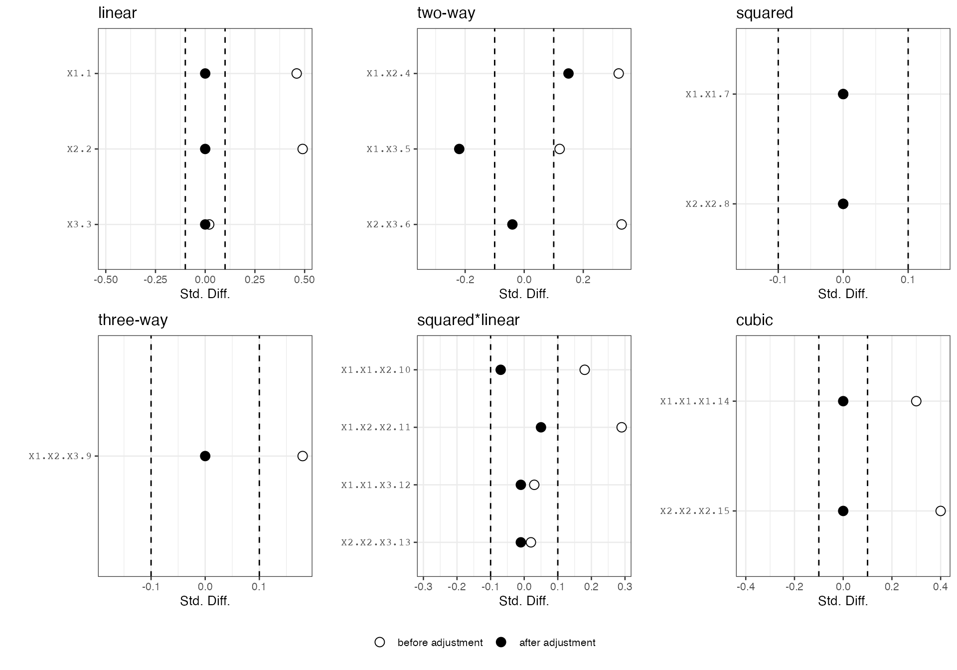
From the above plots, we can see that the linear terms of the covariates are exactly balanced between the treatment and the control groups. We can check the group penalties or penalties applied to each covariate. In this case, the higher-order terms all have relatively high penalties except for two-way interactions, in accordance with the true data generating process.
round(out$group.penalty, 2)
#>         linear        two-way        squared      three-way squared*linear
#>           0.00           1.98           0.00          21.21           6.34
#>          cubic
#>           0.00
round(out$term.penalty, 2)
#>        X1.1        X2.2        X3.3     X1.X2.4     X1.X3.5     X2.X3.6
#>        0.00        0.00        0.00        1.98        1.98        1.98
#>     X1.X1.7     X2.X2.8  X1.X2.X3.9 X1.X1.X2.10 X1.X2.X2.11 X1.X1.X3.12
#>        0.00        0.00       21.21        6.34        6.34        6.34
#> X2.X2.X3.13 X1.X1.X1.14 X2.X2.X2.15
#>        6.34        0.00        0.00
We can also plot the weight distribution for the control units by
specifying type = 'weight' in plot(). We can
see that the weights are quite concentrated around the unit weight.
plot(out, type='weight')
#> sum(weights) normalized to the number of treated units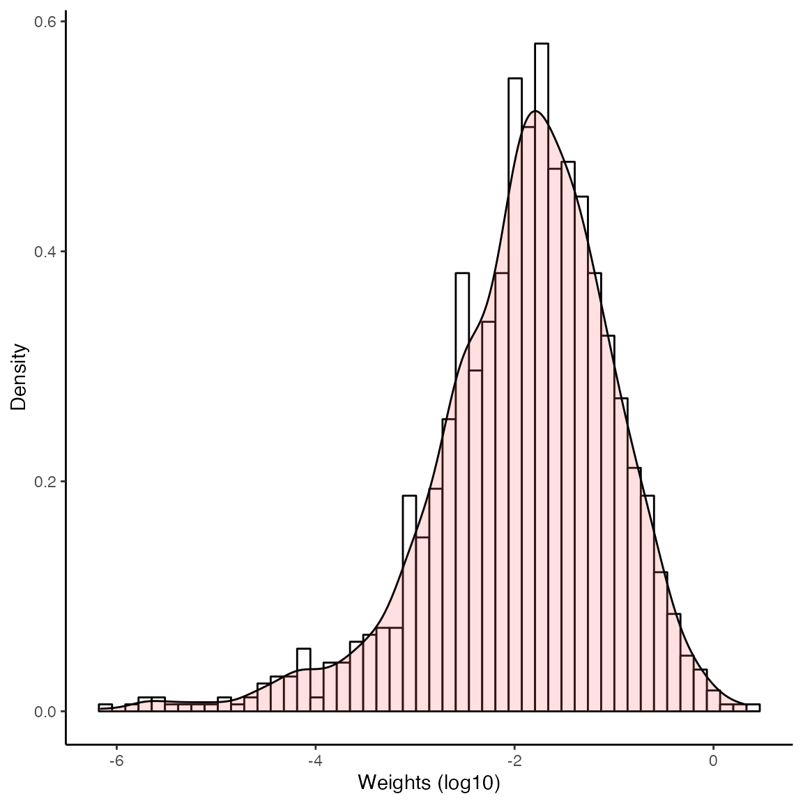
Additional Options
Controlling Exact/Approximate Balancing
Users can manually control which group of covariates to be exactly
balanced and which group to be approximately balanced (via
regularization) by using the group.exact argument. It takes
in a binary vector with length equal to the number of covariate groups,
with 1 indicating exact balance on that group and 0 indicating
approximate balance. Appropriate penalties are then searched through
cross-validation. When using this option, please make that the length of
vector supplied equals the number of groups.
For example, we can ask hbal() to achieve exact balance
on the linear terms and two-way interactions and approximate balance for
the rest:
out <- hbal(Treat = 'D', X = c('X1', 'X2'),  Y = 'Y', data = dat,
            expand.degree = 3, cv = TRUE, group.exact = c(1, 1, 0, 0, 0))
#> Crossvalidation...
summary(out)
#> Call:
#>  hbal(data = dat, Treat = "D", X = c("X1", "X2"), Y = "Y", expand.degree = 3,
#>     cv = TRUE, group.exact = c(1, 1, 0, 0, 0))
#>
#>  Treated Controls
#>      256     1244
#>  Co/Tr Ratio = 4.86
#>
#>  Groups
#>                #Terms Penalty
#> linear              2     0.0
#> two-way             1     0.0
#> squared             2     0.0
#> squared*linear      2     0.1
#> cubic               2    98.8
#>
#>  Balance Table
#>          Tr.Mean Co.Mean W.Co.Mean Std.Diff.(O) Std.Diff.(W)
#> X1          0.35   -0.11      0.35         0.46         0.00
#> X2          0.42   -0.07      0.42         0.49         0.00
#> X1.X2       0.24   -0.10      0.24         0.32         0.00
#> X1.X1       1.01    1.01      1.01         0.00         0.00
#> X2.X2       0.99    0.99      0.99         0.00         0.00
#> X1.X1.X2    0.32   -0.01      0.38         0.18        -0.03
#> X1.X2.X2    0.32   -0.17      0.34         0.29        -0.01
#> X1.X1.X1    0.93   -0.25      1.04         0.30        -0.03
#> X2.X2.X2    1.16   -0.23      0.96         0.40         0.06
User-Supplied Penalties
If researchers have prior knowledge about covariates and would like
to supply specific penalties for each group of covariates, we can do so
by passing a vector of penalties to the group.alpha
argument. For example, we can manually set penalties to be 0 for the the
linear terms and two-way interactions and 100 for other groups:
out <- hbal(Treat = 'D', X = c('X1', 'X2', 'X3'),  Y = 'Y', data = dat,
            expand.degree = 3, group.alpha = c(0, 0, 100, 100, 100, 100))
summary(out)
#> Call:
#>  hbal(data = dat, Treat = "D", X = c("X1", "X2", "X3"), Y = "Y",
#>     expand.degree = 3, group.alpha = c(0, 0, 100, 100, 100, 100))
#>
#>  Treated Controls
#>      256     1244
#>  Co/Tr Ratio = 4.86
#>
#>  Groups
#>                #Terms Penalty
#> linear              3       0
#> two-way             3       0
#> squared             2     100
#> three-way           1     100
#> squared*linear      4     100
#> cubic               2     100
#>
#>  Balance Table
#>          Tr.Mean Co.Mean W.Co.Mean Std.Diff.(O) Std.Diff.(W)
#> X1          0.35   -0.11      0.35         0.46         0.00
#> X2          0.42   -0.07      0.42         0.49         0.00
#> X3          0.52    0.51      0.52         0.02         0.00
#> X1.X2       0.24   -0.10      0.24         0.32         0.00
#> X1.X3       0.07   -0.02      0.07         0.12         0.00
#> X2.X3       0.21   -0.01      0.21         0.33         0.00
#> X1.X1       1.01    1.01      1.18         0.00        -0.12
#> X2.X2       0.99    0.99      1.06         0.00        -0.06
#> X1.X2.X3    0.13    0.00      0.14         0.18        -0.02
#> X1.X1.X2    0.32   -0.01      0.52         0.18        -0.11
#> X1.X2.X2    0.32   -0.17      0.37         0.29        -0.03
#> X1.X1.X3    0.55    0.52      0.58         0.03        -0.03
#> X2.X2.X3    0.50    0.47      0.55         0.02        -0.06
#> X1.X1.X1    0.93   -0.25      1.06         0.30        -0.03
#> X2.X2.X2    1.16   -0.23      1.03         0.40         0.04
Controlling Serial Expansion
Sometimes we may not want to perform serial expansion on all
covariates but instead expand on a select set of covariates, we can do
so by using the X.expand argument to specify the covariates
we want to expand on. For example, we can expand only on
X1:
out <- hbal(Treat = 'D', X = c('X1', 'X2', 'X3'),  Y = 'Y', data = dat,
            expand.degree = 3, X.expand = c('X1', 'X2'))
summary(out)
#> Call:
#>  hbal(data = dat, Treat = "D", X = c("X1", "X2", "X3"), Y = "Y",
#>     X.expand = c("X1", "X2"), expand.degree = 3)
#>
#>  Treated Controls
#>      256     1244
#>  Co/Tr Ratio = 4.86
#>
#>  Groups
#>                #Terms Penalty
#> linear              3       0
#> two-way             1       0
#> squared             2       0
#> squared*linear      2       0
#> cubic               2       0
#>
#>  Balance Table
#>          Tr.Mean Co.Mean W.Co.Mean Std.Diff.(O) Std.Diff.(W)
#> X1          0.35   -0.11      0.35         0.46            0
#> X2          0.42   -0.07      0.42         0.49            0
#> X3          0.52    0.51      0.52         0.02            0
#> X1.X2       0.24   -0.10      0.24         0.32            0
#> X1.X1       1.01    1.01      1.01         0.00            0
#> X2.X2       0.99    0.99      0.99         0.00            0
#> X1.X1.X2    0.32   -0.01      0.32         0.18            0
#> X1.X2.X2    0.32   -0.17      0.32         0.29            0
#> X1.X1.X1    0.93   -0.25      0.93         0.30            0
#> X2.X2.X2    1.16   -0.23      1.16         0.40            0
Selecting Covariates
Performing serial expansion on many covariates can result in a
prohibitive number of covariates that need to be balanced on. In such
cases, users many want to reduce the number of covariates by using the
double selection method by Belloni, Chernozhukov,
and Hansen (2014). This screens the expanded covariates and only
keeps those that are predictive for the treatment assignment or the
outcome. Users can enable double selection by setting
ds = TRUE. In the following case, almost all the
higher-order terms except X1*X2 and X2*X3 are
screened out by the double selection procedure.
out <- hbal(Treat = 'D', X = c('X1', 'X2', 'X3'),  Y = 'Y', data = dat,
            expand.degree = 3, ds = TRUE)
summary(out)
#> Call:
#>  hbal(data = dat, Treat = "D", X = c("X1", "X2", "X3"), Y = "Y",
#>     expand.degree = 3, ds = TRUE)
#>
#>  Treated Controls
#>      256     1244
#>  Co/Tr Ratio = 4.86
#>
#>  Groups
#>         #Terms Penalty
#> linear       2       0
#> two-way      2       0
#>
#>  Balance Table
#>       Tr.Mean Co.Mean W.Co.Mean Std.Diff.(O) Std.Diff.(W)
#> X1       0.35   -0.11      0.35         0.46            0
#> X2       0.42   -0.07      0.41         0.49            0
#> X1.X2    0.24   -0.10      0.24         0.32            0
#> X2.X3    0.21   -0.01      0.21         0.33            0
att(out)
#>    Estimate Std. Error  t value     Pr(>|t|)  CI Lower  CI Upper   DF
#> D 0.4789838 0.07206011 6.647004 4.180629e-11 0.3376341 0.6203335 1494
Keeping/Excluding Covariates
If there are covariates that users would like to keep in the
balancing conditions regardless of whether they are selected in double
selection, we can use the X.keep argument to specify the
covariates to keep. On the other hand, if a priori we know some
combinations of the covariates are nonsensical, we can exclude them
explicitly by using the exclude argument. For example, we
can exclude any interaction that involves X1 and
X2:
out <- hbal(Treat = 'D', X = c('X1', 'X2', 'X3'),  Y = 'Y', data = dat,
            expand.degree = 3, exclude = list(c('X1', 'X2')))
summary(out) # X1.X2 and X1.X1.X2 removed from balancing scheme
#> Call:
#>  hbal(data = dat, Treat = "D", X = c("X1", "X2", "X3"), Y = "Y",
#>     expand.degree = 3, exclude = list(c("X1", "X2")))
#>
#>  Treated Controls
#>      256     1244
#>  Co/Tr Ratio = 4.86
#>
#>  Groups
#>                #Terms Penalty
#> linear              3       0
#> two-way             2       0
#> squared             2       0
#> squared*linear      2       0
#> cubic               2       0
#>
#>  Balance Table
#>          Tr.Mean Co.Mean W.Co.Mean Std.Diff.(O) Std.Diff.(W)
#> X1          0.35   -0.11      0.35         0.46            0
#> X2          0.42   -0.07      0.42         0.49            0
#> X3          0.52    0.51      0.52         0.02            0
#> X1.X3       0.07   -0.02      0.07         0.12            0
#> X2.X3       0.21   -0.01      0.21         0.33            0
#> X1.X1       1.01    1.01      1.01         0.00            0
#> X2.X2       0.99    0.99      0.99         0.00            0
#> X1.X1.X3    0.55    0.52      0.55         0.03            0
#> X2.X2.X3    0.50    0.47      0.50         0.02            0
#> X1.X1.X1    0.93   -0.25      0.93         0.30            0
#> X2.X2.X2    1.16   -0.23      1.16         0.40            0
att(out)
#>   Estimate Std. Error  t value    Pr(>|t|)  CI Lower  CI Upper   DF
#> D 0.485784 0.07169999 6.775232 1.78421e-11 0.3451402 0.6264279 1487
Example 1: Lalonde Data
To show the use of habl in practice, here we use habl on a dataset that contains the subset of the LaLonde (1986) dataset from Dehejia and Wahba (1999) and the Panel Study of Income Dynamics (PSID-1), which is also shipped with hbal.
data(hbal)
head(lalonde)
#>   nsw age educ black hisp married re74 re75 re78 u74 u75 u78 nodegr
#> 1   0  47   12     0    0       0    0    0    0   1   1   1      0
#> 2   0  50   12     1    0       1    0    0    0   1   1   1      0
#> 3   0  44   12     0    0       0    0    0    0   1   1   1      0
#> 4   0  28   12     1    0       1    0    0    0   1   1   1      0
#> 5   0  54   12     0    0       1    0    0    0   1   1   1      0
#> 6   0  55   12     0    1       1    0    0    0   1   1   1      0
First, we adjust for the linear terms only:
xvars <- c("age","black","educ","hisp","married","re74","re75","nodegr","u74","u75") # covariates
# hbal w/ level terms only
hbal.out <- hbal(Treat = 'nsw', X = xvars,  Y = 're78', data = lalonde)
summary(hbal.out)
#> Call:
#>  hbal(data = lalonde, Treat = "nsw", X = xvars, Y = "re78")
#>
#>  Treated Controls
#>      185     2490
#>  Co/Tr Ratio = 13.46
#>
#>  Groups
#>        #Terms Penalty
#> linear     10       0
#>
#>  Balance Table
#>       Tr.Mean  Co.Mean W.Co.Mean Std.Diff.(O) Std.Diff.(W)
#> age     25.82    34.85     25.82        -0.86            0
#> black   10.35    12.12     10.35        -0.58            0
#> educ     0.84     0.25      0.84         1.30            0
#> hisp     0.06     0.03      0.06         0.15            0
#> marri    0.19     0.87      0.19        -1.76            0
#> re74  2095.57 19428.75   2100.16        -1.26            0
#> re75  1532.06 19063.34   1536.82        -1.26            0
#> nodeg    0.71     0.09      0.71         1.85            0
#> u74      0.60     0.10      0.60         1.46            0
#> age0     0.71     0.31      0.71         0.85            0
att(hbal.out)
#>     Estimate Std. Error  t value     Pr(>|t|) CI Lower CI Upper   DF
#> nsw 2423.165   719.4805 3.367937 0.0007680966 1012.368 3833.962 2663
Adding higher-order terms makes the treatment effect estimate closer
to the experimental benchmark (~$1800). As a result of cross-validation,
no penalty is imposed on the linear and squared terms. Note that
exclude=list(c("educ", "nodegr")) removes the nonsensical
interaction between educ and nodegr.
hbal.full.out <- hbal(Treat = 'nsw', X = xvars, Y = 're78', data = lalonde,
                      expand.degree = 2, cv = TRUE, exclude=list(c("educ", "nodegr")))
#> Crossvalidation...
summary(hbal.full.out)
#> Call:
#>  hbal(data = lalonde, Treat = "nsw", X = xvars, Y = "re78", expand.degree = 2,
#>     cv = TRUE, exclude = list(c("educ", "nodegr")))
#>
#>  Treated Controls
#>      185     2490
#>  Co/Tr Ratio = 13.46
#>
#>  Groups
#>         #Terms Penalty
#> linear      10       0
#> squared      4       0
#> two-way     42     100
#>
#>  Balance Table
#>                 Tr.Mean      Co.Mean   W.Co.Mean Std.Diff.(O) Std.Diff.(W)
#> age               25.82        34.85       25.82        -0.86         0.00
#> black             10.35        12.12       10.35        -0.58         0.00
#> educ               0.84         0.25        0.84         1.30         0.00
#> hisp               0.06         0.03        0.06         0.15         0.00
#> marri              0.19         0.87        0.19        -1.76         0.00
#> re74            2095.57     19428.75     2095.64        -1.26         0.00
#> re75            1532.06     19063.34     1532.08        -1.26         0.00
#> nodeg              0.71         0.09        0.71         1.85         0.00
#> u74                0.60         0.10        0.60         1.46         0.00
#> age0               0.71         0.31        0.71         0.85         0.00
#> age.age          717.39      1323.53      726.97        -0.79        -0.01
#> black.black      111.06       156.32      112.06        -0.64        -0.01
#> re74.re74   28141434.44 557148332.57 25567475.07        -0.62         0.00
#> re75.re75   12654752.23 548213776.79 12138371.63        -0.60         0.00
#> age.black        266.98       414.70      261.76        -0.95         0.03
#> age.educ          21.91         8.56       21.26         0.84         0.04
#> black.educ         8.70         2.60        8.43         1.23         0.05
#> age.hisp           1.36         1.16        1.63         0.03        -0.04
#> black.hisp         0.58         0.35        0.74         0.11        -0.08
#> age.marri          5.56        30.90        6.50        -1.53        -0.06
#> black.marri        1.96        10.47        1.94        -1.57         0.00
#> educ.marri         0.16         0.20        0.12        -0.10         0.09
#> hisp.marri         0.02         0.03        0.01        -0.08         0.01
#> age.re74       54074.04    704912.21    53890.91        -1.07         0.00
#> black.re74     22898.73    248073.37    22654.36        -1.08         0.00
#> educ.re74       1817.20      3646.09     1703.81        -0.24         0.01
#> hisp.re74        151.40       589.15      132.10        -0.12         0.01
#> marri.re74       760.63     17578.61      834.92        -1.15        -0.01
#> age.re75       41167.28    688282.61    38042.18        -1.07         0.01
#> black.re75     15880.57    244584.33    16095.74        -1.09         0.00
#> educ.re75       1257.04      3502.23     1316.30        -0.30        -0.01
#> hisp.re75        153.73       511.72       46.78        -0.10         0.03
#> marri.re75       654.34     17200.24      485.94        -1.13         0.01
#> re74.re75   13118590.79 523653961.37 11715080.77        -0.62         0.00
#> age.nodeg         18.78         3.50       18.54         1.22         0.02
#> black.nodeg        7.26         1.01        7.35         1.60        -0.02
#> educ.nodeg         0.60         0.01        0.59         2.57         0.05
#> hisp.nodeg         0.03         0.00        0.05         0.39        -0.19
#> marri.nodeg        0.11         0.07        0.11         0.15         0.03
#> re75.nodeg       307.44       372.31      286.15        -0.02         0.01
#> age.u74           15.98         3.99       16.38         0.93        -0.03
#> black.u74          6.15         1.15        6.31         1.26        -0.04
#> educ.u74           0.52         0.02        0.52         2.15        -0.01
#> hisp.u74           0.03         0.01        0.02         0.27         0.12
#> marri.u74          0.09         0.09        0.12         0.00        -0.12
#> re74.u74          43.85       483.27      361.33        -0.13        -0.10
#> nodeg.u74          0.59         0.07        0.53         1.74         0.18
#> age.age0          17.97        11.83       18.45         0.33        -0.03
#> black.age0         6.71         2.62        6.64         0.95         0.02
#> educ.age0          0.61         0.13        0.66         1.28        -0.13
#> hisp.age0          0.05         0.01        0.02         0.27         0.23
#> marri.age0         0.14         0.26        0.11        -0.28         0.07
#> re74.age0       1094.15      4511.11     1198.46        -0.40        -0.01
#> re75.age0       1134.96      4272.56     1013.44        -0.37         0.01
#> nodeg.age0         0.52         0.03        0.51         2.01         0.05
#> u74.age0           0.43         0.04        0.43         1.58         0.00
att(hbal.full.out)
#>     Estimate Std. Error  t value    Pr(>|t|) CI Lower CI Upper   DF
#> nsw 2081.452   725.9504 2.867209 0.004174207 657.9566 3504.947 2617
We can check the penalties applied to each group and the cavariate balance before and after balancing.
hbal.full.out$group.penalty
#>       linear      squared      two-way
#> 0.000000e+00 7.997239e-03 1.000000e+02
plot(hbal.full.out)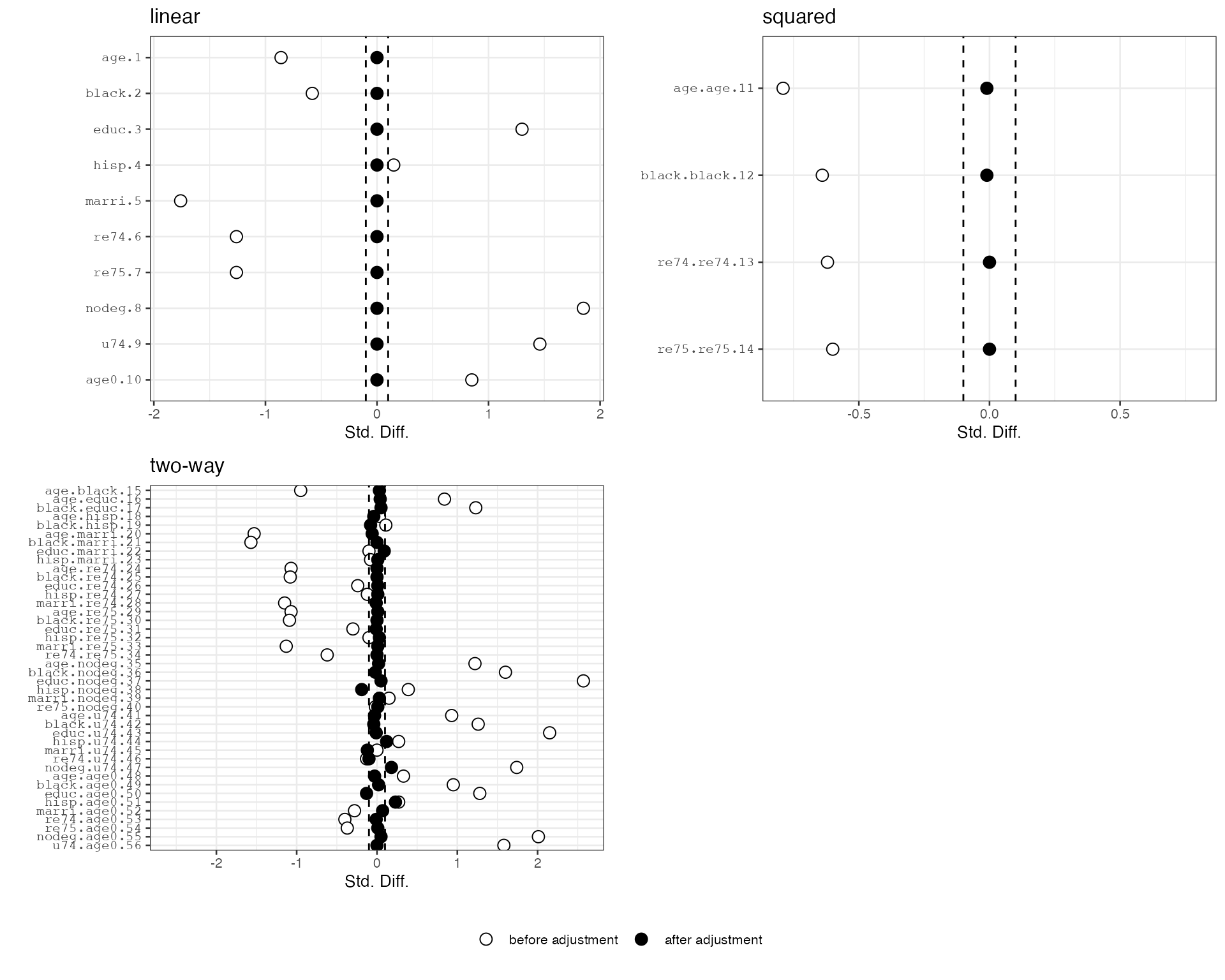
Example 2: Black and Owens (2016)
The second example comes from Black and Owens
(2016), in which the authors study the effect of promotion
prospect to the Supreme Court on the behavior of circuit court judges.
Here we focus on whether circuit court judges who are on the shortlist
to fill Supreme Court vacancies (“contenders”) ruled in line with the
president as the outcome of interest. We load the dataset
contenderJudges, which is shipped with
hbal.
data(hbal)First, we take a look at the data structure. The outcome variable is
presIdeoVote and the treatment variable is
treatFinal0, indicating whether there was a Supreme Court
vacancy at the time. There are also 7 covariates on judge and court
characteristics and a variable judge that indicates the
judges’ names.
str(contenderJudges)
#> 'data.frame':    10171 obs. of  10 variables:
#>  $ presIdeoVote: int  0 1 1 1 1 0 0 0 1 0 ...
#>  $ treatFinal0 : int  1 1 1 1 1 1 1 1 1 1 ...
#>  $ judgeJCS    : num  0.28 0.581 0.199 0.406 -0.341 ...
#>  $ presDist    : num  0.0019 0.0552 0.3137 0.2302 0.9772 ...
#>  $ panelDistJCS: num  0.0392 0.562 0.2485 0.4625 0.491 ...
#>  $ circmed     : num  0.0315 0.581 0.0375 0.013 0.047 ...
#>  $ sctmed      : num  0.227 0.122 -0.359 0.122 0.122 ...
#>  $ coarevtc    : int  0 0 0 1 1 1 0 1 0 1 ...
#>  $ casepub     : int  1 1 1 1 1 1 1 1 1 1 ...
#>  $ judge       : Factor w/ 68 levels "Alfred T. Goodwin",..: 34 31 9 4 3 59 67 52 16 34 ...
We can estimate the effect of Supreme Court vacancy on judges’ rulings while controlling for functions of the covariates (to the second order). We see that contender judges are more likely to rule in line with the ideology of the sitting president during a Supreme Court vacancy.
xvars <- c("judgeJCS", "presDist", "panelDistJCS", "circmed", "sctmed", "coarevtc", "casepub")
out <- hbal(Treat = 'treatFinal0', X = xvars, Y = 'presIdeoVote', data = contenderJudges,
            expand.degree = 2, cv = TRUE)
#> Crossvalidation...
summary(out)
#> Call:
#>  hbal(data = contenderJudges, Treat = "treatFinal0", X = xvars,
#>     Y = "presIdeoVote", expand.degree = 2, cv = TRUE)
#>
#>  Treated Controls
#>     4490     5681
#>  Co/Tr Ratio = 1.27
#>
#>  Groups
#>         #Terms Penalty
#> linear       7     0.0
#> squared      5     0.3
#> two-way     21     0.0
#>
#>  Balance Table
#>             Tr.Mean Co.Mean W.Co.Mean Std.Diff.(O) Std.Diff.(W)
#> judge          0.16    0.07      0.16         0.28         0.00
#> presD          0.17    0.45      0.17        -0.91         0.00
#> panel          0.34    0.29      0.34         0.23         0.00
#> circm          0.14    0.00      0.14         0.50         0.00
#> sctme          0.01    0.03      0.01        -0.07         0.00
#> coare          0.28    0.31      0.28        -0.07         0.00
#> casep          0.61    0.84      0.61        -0.53         0.00
#> judge.judge    0.13    0.12      0.14         0.10        -0.09
#> presD.presD    0.06    0.31      0.07        -0.84        -0.02
#> panel.panel    0.18    0.14      0.18         0.18        -0.03
#> circm.circm    0.08    0.08      0.09         0.01        -0.09
#> sctme.sctme    0.04    0.02      0.03         0.40         0.17
#> judge.presD    0.02    0.02      0.02         0.02        -0.03
#> judge.panel    0.05    0.03      0.05         0.15         0.00
#> presD.panel    0.04    0.13      0.05        -0.59        -0.02
#> judge.circm    0.05    0.05      0.05         0.02        -0.02
#> presD.circm    0.01    0.00      0.01         0.08         0.00
#> panel.circm    0.05    0.01      0.05         0.37         0.00
#> judge.sctme   -0.02    0.01     -0.02        -0.54        -0.07
#> presD.sctme   -0.01    0.02     -0.01        -0.41         0.00
#> panel.sctme    0.01    0.01      0.01         0.00        -0.03
#> circm.sctme    0.01    0.01      0.01        -0.08        -0.01
#> judge.coare    0.05    0.02      0.05         0.13         0.00
#> presD.coare    0.05    0.14      0.05        -0.39         0.00
#> panel.coare    0.10    0.09      0.10         0.04        -0.01
#> circm.coare    0.03    0.00      0.03         0.21         0.00
#> sctme.coare    0.01    0.01      0.01        -0.02         0.01
#> judge.casep    0.10    0.04      0.09         0.23         0.06
#> presD.casep    0.12    0.37      0.12        -0.83        -0.02
#> panel.casep    0.21    0.24      0.21        -0.09         0.03
#> circm.casep    0.05   -0.02      0.05         0.30         0.00
#> sctme.casep    0.00    0.01      0.00        -0.09         0.03
#> coare.casep    0.22    0.30      0.23        -0.16        -0.01
att(out)
#>               Estimate Std. Error  t value     Pr(>|t|)   CI Lower   CI Upper
#> treatFinal0 0.04317827 0.01256806 3.435556 0.0005937101 0.01854238 0.06781416
#>                DF
#> treatFinal0 10136
We can further check covariate balance before and after balancing by checking the balance plots. Here we see that the linear terms are exactly balanced between the treatment and the control groups. Imbalance among higher-order terms and interactions are also significantly reduced.
plot(out)