Tutorial
tutorial.RmdSince gsynth is a wrapper package for fect, which is likely to be better maintained, we recommend users use fect (User Manual) directly for most purposes. We maintain this website and package solely for backward compatibility.
Two datasets simdata and turnout are shipped with the gsynth package. Load these two datasets:
library(gsynth)
#> ## Since v.1.3.0, *gsynth* is a wrapper of the *fect* package.
#> ## Comments and suggestions -> yiqingxu@stanford.edu.
data(gsynth)
ls()
#> [1] "simdata" "turnout"
Block DID
We start with the first example, a simulated dataset described in the paper. There are 5 treated units, 45 control units, and 30 time periods. The treatment kicks at Period 21 for all treated units, hence, a multiperiod block DID setting.
head(simdata)
#>    id time         Y D        X1         X2 eff      error mu       alpha
#> 1 101    1  6.210998 0 0.3776736 -0.1732470   0  0.2982276  5 -0.06052364
#> 2 101    2  4.027106 0 1.7332009 -0.4945009   0  0.6365697  5 -0.06052364
#> 3 101    3  8.877187 0 1.8580159  0.4984432   0 -0.4837806  5 -0.06052364
#> 4 101    4 11.515346 0 1.3943369  1.1272713   0  0.5168620  5 -0.06052364
#> 5 101    5  5.971526 0 2.3636963 -0.1535215   0  0.3689645  5 -0.06052364
#> 6 101    6  8.237905 0 0.5370867  0.8774397   0 -0.2153805  5 -0.06052364
#>           xi          F1          L1           F2         L2
#> 1  1.1313372  0.25331851 -0.04303273  0.005764186 -0.8804667
#> 2 -1.4606401 -0.02854676 -0.04303273  0.385280401 -0.8804667
#> 3  0.7399475 -0.04287046 -0.04303273 -0.370660032 -0.8804667
#> 4  1.9091036  1.36860228 -0.04303273  0.644376549 -0.8804667
#> 5 -1.4438932 -0.22577099 -0.04303273 -0.220486562 -0.8804667
#> 6  0.7017843  1.51647060 -0.04303273  0.331781964 -0.8804667
Visualizing data
Before we conduct any statistical analysis, it is helpful to visualize the data structure and/or spot missing values (if there are any). We can easily do so with the help of the panelView package. The following figure shows that: (1) there are 5 treated units and 45 control units; (2) the treated units start to be treated in period 21; and (3) there are no missing values, which is a rare case.
## devtools::install_github('xuyiqing/panelView')   # if not already installed
library(panelView)
#> ## See bit.ly/panelview4r for more info.
#> ## Report bugs -> yiqingxu@stanford.edu.
panelview(Y ~ D, data = simdata, index = c("id","time"), pre.post = TRUE) 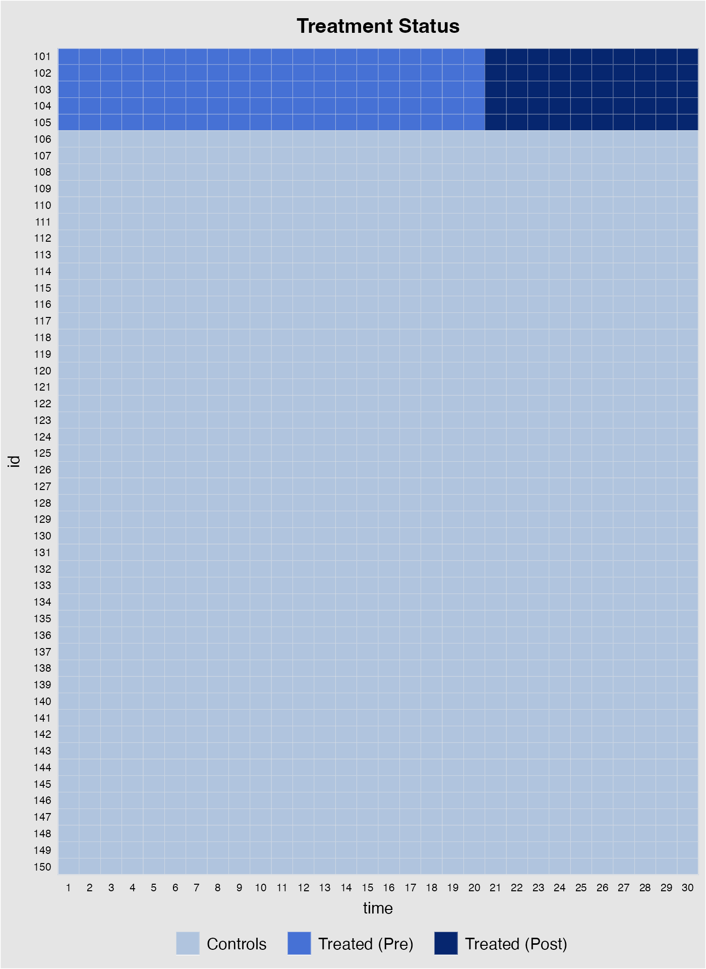
The following line of code visualizes the outcome variable; different colors correspond to different treatment status.
Estimation
We estimate the model only using information of the outcome variable , the treatment indicator , and two observed covariates and (as well as the group indicators and ).
Now we formally run the gsynth algorithm proposed by
Xu (2017). The first variable on the
right-hand-side of the formula is a binary treatment indicator. The rest
of the right-hand-side variables serve as controls. The
index option specifies the unit and time indicators.
The force option (“none”, “unit”, “time”, and “two-way”)
specifies the additive component(s) of the fixed effects included in the
model. The default option is “unit” (including additive unit fixed
effects). A cross-validation procedure is provided (when
CV = TRUE) to select the number of unobserved factors
within the interval of r=c(0,5). When cross-validation is
switched off, the first element in r will be set as the
number of factors.
When the uncertainty estimates are needed, set
se = TRUE. When the number of treated units is small, a
parametric bootstrap procedure is preferred, i.e.,
inference = "parametric". Alternatively, one can use a
non-parametric bootstrap procedure by setting
inference = "nonparametric"; it only works well when the
treatment group is relatively large,
e.g. ).
The number of bootstrap runs is set by nboots.
When dealing with clustered data, for example, panel data with
regionally clustered units, one can use the cluster bootstrap procedure
by specifying name of the cluster variable in option cl.
For example, cl = "state" for city-level data.
system.time(
    out <- gsynth(Y ~ D + X1 + X2, data = simdata,
                  index = c("id","time"), force = "two-way",
                  CV = TRUE, r = c(0, 5), se = TRUE,
                  inference = "parametric", nboots = 1000,
                  parallel = FALSE)
)
#> Cross-validating ...
#> Criterion: Mean Squared Prediction Error
#> Interactive fixed effects model...
#> Cross-validating ...
#> r = 0; sigma2 = 1.84865; IC = 1.02023; PC = 1.74458; MSPE = 2.37280
#> r = 1; sigma2 = 1.51541; IC = 1.20588; PC = 1.99818; MSPE = 1.71743
#> r = 2; sigma2 = 0.99737; IC = 1.16130; PC = 1.69046; MSPE = 1.14540
#> *
#> r = 3; sigma2 = 0.94664; IC = 1.47216; PC = 1.96215; MSPE = 1.15032
#> r = 4; sigma2 = 0.89411; IC = 1.76745; PC = 2.19241; MSPE = 1.21397
#> r = 5; sigma2 = 0.85060; IC = 2.05928; PC = 2.40964; MSPE = 1.23876
#>
#>  r* = 2
#>
#> Parametric Bootstrap
#> Simulating errors ...
#> Can't calculate the F statistic because of insufficient treated units.
#>    user  system elapsed
#>  10.652   0.121  10.805
Because the core function of gsynth is written in C++, the algorithm runs relatively fast. The entire procedure (including cross-validation and 1,000 bootstrap runs) takes about 6 seconds on an iMac (2016 model).
The algorithm prints out the results automatically.
sigma2 stands for the estimated variance of the error term;
IC represents the Bayesian Information Criterion; and
MPSE is the Mean Squared Prediction Error. The
cross-validation procedure selects an
that minimizes the MSPE.
Users can use the print function to visualize the
result or retrieve the numbers by directly accessing the gsynth object.
est.att reports the average treatment effect on the treated
(ATT) by period; est.avg shows the ATT averaged over all
periods; and est.beta reports the coefficients of the
time-varying covariates. Treatment effect estimates from each bootstrap
run is stored in eff.boot, an array whose dimension =
(#time periods * #treated * #bootstrap runs).
out$est.att
#>              ATT      S.E.   CI.lower    CI.upper      p.value count
#> -19  0.392159788 0.5535722 -0.6928219  1.47714145 4.786866e-01     5
#> -18  0.276547958 0.4636046 -0.6321003  1.18519619 5.508300e-01     5
#> -17 -0.275392926 0.5283828 -1.3110041  0.76021827 6.022277e-01     5
#> -16  0.441201288 0.4449525 -0.4308896  1.31329213 3.214076e-01     5
#> -15 -0.889595124 0.4960590 -1.8618528  0.08266256 7.292091e-02     5
#> -14  0.593890957 0.4546032 -0.2971149  1.48489678 1.914185e-01     5
#> -13  0.528749012 0.4048114 -0.2646668  1.32216482 1.914977e-01     5
#> -12  0.171568737 0.5501494 -0.9067043  1.24984174 7.551481e-01     5
#> -11  0.610832288 0.5038120 -0.3766212  1.59828574 2.253513e-01     5
#> -10  0.170597468 0.4640166 -0.7388584  1.08005329 7.131314e-01     5
#> -9  -0.271891657 0.5884914 -1.4253136  0.88153024 6.440708e-01     5
#> -8   0.094842558 0.4892671 -0.8641033  1.05378841 8.462963e-01     5
#> -7  -0.651975701 0.5412546 -1.7128152  0.40886381 2.283717e-01     5
#> -6   0.573686472 0.4983252 -0.4030129  1.55038584 2.496380e-01     5
#> -5  -0.469685905 0.4720492 -1.3948853  0.45551352 3.197394e-01     5
#> -4  -0.077766449 0.5751820 -1.2051024  1.04956955 8.924512e-01     5
#> -3  -0.141784521 0.5513196 -1.2223511  0.93878204 7.970452e-01     5
#> -2  -0.157100323 0.4096073 -0.9599159  0.64571526 7.013203e-01     5
#> -1  -0.915575087 0.5267280 -1.9479430  0.11679281 8.217007e-02     5
#> 0   -0.003308833 0.3507817 -0.6908282  0.68421057 9.924739e-01     5
#> 1    1.235962010 0.7243851 -0.1838067  2.65573073 8.796670e-02     5
#> 2    1.630264312 0.5633958  0.5260289  2.73449973 3.808050e-03     5
#> 3    2.712177702 0.5934660  1.5490058  3.87534964 4.875745e-06     5
#> 4    3.466757691 0.7186178  2.0582926  4.87522275 1.405648e-06     5
#> 5    5.740132310 0.5594497  4.6436310  6.83663366 0.000000e+00     5
#> 6    5.280034526 0.5767505  4.1496243  6.41044476 0.000000e+00     5
#> 7    8.436484821 0.4670150  7.5211522  9.35181743 0.000000e+00     5
#> 8    7.839901526 0.6406018  6.5843452  9.09545789 0.000000e+00     5
#> 9    9.455114684 0.5239232  8.4282440 10.48198537 0.000000e+00     5
#> 10   9.638509457 0.4916055  8.6749803 10.60203857 0.000000e+00     5
out$est.avg
#>       ATT.avg      S.E. CI.lower CI.upper p.value
#> [1,] 5.543534 0.2655813 5.023004 6.064064       0
out$est.beta
#>        Coef       S.E.  CI.lower CI.upper p.value
#> X1 1.021890 0.03117269 0.9607928 1.082988       0
#> X2 3.052994 0.02895597 2.9962417 3.109747       0
Parallel computing will speed up the bootstrap procedure
significantly. When parallel = TRUE (default) and
cores options are omitted, the algorithm will detect the
number of available cores on your computer automatically. (Warning: it
may consume most of your computer’s computational power if all cores are
being used.) Starting from v1.3.0, we use the doRNG
package to ensure the reproducibility of results under parallel
computing.
system.time(
out <- gsynth(Y ~ D + X1 + X2, data = simdata,
              index = c("id","time"), force = "two-way",
              CV = TRUE, r = c(0, 5), se = TRUE,
              inference = "parametric", nboots = 1000,
              parallel = TRUE, cores = 10)
)
#> Parallel computing ...
#> Cross-validating ...
#> Criterion: Mean Squared Prediction Error
#> Interactive fixed effects model...
#> Cross-validating ...
#> r = 0; sigma2 = 1.84865; IC = 1.02023; PC = 1.74458; MSPE = 2.37280
#> r = 1; sigma2 = 1.51541; IC = 1.20588; PC = 1.99818; MSPE = 1.71743
#> r = 2; sigma2 = 0.99737; IC = 1.16130; PC = 1.69046; MSPE = 1.14540
#> *
#> r = 3; sigma2 = 0.94664; IC = 1.47216; PC = 1.96215; MSPE = 1.15032
#> r = 4; sigma2 = 0.89411; IC = 1.76745; PC = 2.19241; MSPE = 1.21397
#> r = 5; sigma2 = 0.85060; IC = 2.05928; PC = 2.40964; MSPE = 1.23876
#>
#>  r* = 2
#>
#> Parametric Bootstrap
#> Simulating errors ...
#> Can't calculate the F statistic because of insufficient treated units.
#>    user  system elapsed
#>   1.572   0.327   4.024
print(out)
#> Call:
#> gsynth(formula = Y ~ D + X1 + X2, data = simdata, index = c("id",
#>     "time"), force = "two-way", r = c(0, 5), CV = TRUE, se = TRUE,
#>     nboots = 1000, inference = "parametric", parallel = TRUE,
#>     cores = 10, vartype = "parametric")
#>
#> Average Treatment Effect on the Treated:
#>      ATT.avg   S.E. CI.lower CI.upper p.value
#> [1,]   5.544 0.2747    5.005    6.082       0
#>
#>    ~ by Period (including Pre-treatment Periods):
#>           ATT   S.E. CI.lower CI.upper   p.value count
#> -19  0.392160 0.5775  -0.7397  1.52404 4.971e-01     5
#> -18  0.276548 0.4466  -0.5987  1.15182 5.357e-01     5
#> -17 -0.275393 0.5565  -1.3661  0.81535 6.207e-01     5
#> -16  0.441201 0.4269  -0.3954  1.27783 3.013e-01     5
#> -15 -0.889595 0.5115  -1.8922  0.11297 8.202e-02     5
#> -14  0.593891 0.4900  -0.3665  1.55425 2.255e-01     5
#> -13  0.528749 0.3968  -0.2490  1.30649 1.827e-01     5
#> -12  0.171569 0.5485  -0.9035  1.24665 7.544e-01     5
#> -11  0.610832 0.4589  -0.2887  1.51033 1.832e-01     5
#> -10  0.170597 0.4419  -0.6955  1.03671 6.995e-01     5
#> -9  -0.271892 0.5919  -1.4320  0.88818 6.460e-01     5
#> -8   0.094843 0.4733  -0.8328  1.02253 8.412e-01     5
#> -7  -0.651976 0.5778  -1.7844  0.48045 2.591e-01     5
#> -6   0.573686 0.4957  -0.3978  1.54519 2.471e-01     5
#> -5  -0.469686 0.5479  -1.5435  0.60418 3.913e-01     5
#> -4  -0.077766 0.5765  -1.2077  1.05217 8.927e-01     5
#> -3  -0.141785 0.5647  -1.2487  0.96510 8.018e-01     5
#> -2  -0.157100 0.3955  -0.9323  0.61809 6.912e-01     5
#> -1  -0.915575 0.5103  -1.9157  0.08454 7.277e-02     5
#> 0   -0.003309 0.3491  -0.6876  0.68094 9.924e-01     5
#> 1    1.235962 0.7129  -0.1614  2.63331 8.299e-02     5
#> 2    1.630264 0.5677   0.5177  2.74287 4.081e-03     5
#> 3    2.712178 0.5926   1.5506  3.87371 4.728e-06     5
#> 4    3.466758 0.6964   2.1018  4.83176 6.431e-07     5
#> 5    5.740132 0.5548   4.6527  6.82754 0.000e+00     5
#> 6    5.280035 0.5508   4.2004  6.35967 0.000e+00     5
#> 7    8.436485 0.4533   7.5480  9.32501 0.000e+00     5
#> 8    7.839902 0.6361   6.5932  9.08657 0.000e+00     5
#> 9    9.455115 0.5500   8.3772 10.53307 0.000e+00     5
#> 10   9.638509 0.4858   8.6863 10.59067 0.000e+00     5
#>
#> Coefficients for the Covariates:
#>     Coef    S.E. CI.lower CI.upper p.value
#> X1 1.022 0.03055    0.962    1.082       0
#> X2 3.053 0.02956    2.995    3.111       0
gsynth also incoporates jackknife method for uncertainty estimates.
out2 <- gsynth(Y ~ D + X1 + X2, data = simdata,
               index = c("id","time"), force = "two-way",
               CV = FALSE, r = c(2, 5), se = TRUE,
               inference = "jackknife",
               parallel = TRUE, cores = 10)
#> Parallel computing ...
#> Can't calculate the F statistic because of insufficient treated units.

print(out2)
#> Call:
#> gsynth(formula = Y ~ D + X1 + X2, data = simdata, index = c("id",
#>     "time"), force = "two-way", r = c(2, 5), CV = FALSE, se = TRUE,
#>     inference = "jackknife", parallel = TRUE, cores = 10, vartype = "jackknife")
#>
#> Average Treatment Effect on the Treated:
#>      ATT.avg   S.E. CI.lower CI.upper p.value
#> [1,]   5.544 0.2519     5.05    6.037       0
#>
#>    ~ by Period (including Pre-treatment Periods):
#>           ATT   S.E. CI.lower CI.upper   p.value count
#> -19  0.392160 0.4951  -0.5783   1.3626 4.283e-01     5
#> -18  0.276548 0.3577  -0.4245   0.9775 4.394e-01     5
#> -17 -0.275393 0.5614  -1.3757   0.8249 6.238e-01     5
#> -16  0.441201 0.3173  -0.1807   1.0632 1.644e-01     5
#> -15 -0.889595 0.5078  -1.8849   0.1057 7.982e-02     5
#> -14  0.593891 0.7150  -0.8074   1.9952 4.062e-01     5
#> -13  0.528749 0.3266  -0.1113   1.1688 1.054e-01     5
#> -12  0.171569 0.3755  -0.5644   0.9075 6.477e-01     5
#> -11  0.610832 0.5762  -0.5185   1.7402 2.891e-01     5
#> -10  0.170597 0.5973  -1.0001   1.3413 7.752e-01     5
#> -9  -0.271892 0.5087  -1.2689   0.7251 5.930e-01     5
#> -8   0.094843 0.5207  -0.9257   1.1154 8.555e-01     5
#> -7  -0.651976 0.6346  -1.8958   0.5918 3.042e-01     5
#> -6   0.573686 0.3862  -0.1832   1.3305 1.374e-01     5
#> -5  -0.469686 0.3970  -1.2478   0.3084 2.368e-01     5
#> -4  -0.077766 0.5818  -1.2181   1.0626 8.937e-01     5
#> -3  -0.141785 0.5423  -1.2046   0.9211 7.937e-01     5
#> -2  -0.157100 0.5757  -1.2855   0.9713 7.850e-01     5
#> -1  -0.915575 0.2753  -1.4552  -0.3759 8.834e-04     5
#> 0   -0.003309 0.2547  -0.5025   0.4959 9.896e-01     5
#> 1    1.235962 1.0021  -0.7281   3.2001 2.174e-01     5
#> 2    1.630264 0.9725  -0.2759   3.5364 9.368e-02     5
#> 3    2.712178 0.7198   1.3014   4.1230 1.646e-04     5
#> 4    3.466758 0.9010   1.7009   5.2326 1.192e-04     5
#> 5    5.740132 0.8594   4.0558   7.4245 2.400e-11     5
#> 6    5.280035 0.4326   4.4322   6.1279 0.000e+00     5
#> 7    8.436485 0.6599   7.1431   9.7299 0.000e+00     5
#> 8    7.839902 0.7033   6.4615   9.2183 0.000e+00     5
#> 9    9.455115 0.5773   8.3236  10.5866 0.000e+00     5
#> 10   9.638509 1.1351   7.4137  11.8633 0.000e+00     5
#>
#> Coefficients for the Covariates:
#>     Coef    S.E. CI.lower CI.upper p.value
#> X1 1.022 0.02870   0.9656    1.078       0
#> X2 3.053 0.03302   2.9883    3.118       0
Cumulative effcts
Sometimes, researchers may be interested in cumulative treatment
effects, such as cumulative abnormal returns in an event study. We
provide a simple function, effect, to calculate cumulative
treatment effects. You can specify a period of interest using the
period option. If left blank, cumulative treatment effects
for the entire post-treatment period will be calculated.
cumu1 <- effect(out, cumu = TRUE, id = NULL)
cumu1$effect.est.att
#>          ATT      S.E.   CI.lower  CI.upper      p.value
#> 1   1.235962 0.7129449 -0.1630793  2.635003 8.329742e-02
#> 2   2.866226 1.0131816  0.8780181  4.854434 4.763753e-03
#> 3   5.578404 1.1878691  3.2473992  7.909409 3.021327e-06
#> 4   9.045162 1.5232021  6.0561191 12.034204 3.971832e-09
#> 5  14.785294 1.8067045 11.2399228 18.330665 8.334993e-16
#> 6  20.065329 1.8273804 16.4793842 23.651273 1.460640e-26
#> 7  28.501813 1.9786081 24.6191087 32.384518 6.944946e-43
#> 8  36.341715 2.3036538 31.8211596 40.862270 3.136246e-50
#> 9  45.796830 2.6169418 40.6614963 50.932163 5.112499e-60
#> 10 55.435339 2.7466887 50.0453980 60.825280 3.035739e-76
plot(cumu1)
You can also calculate the ATT for a sub-group by specifying unit
names in the id option. By setting
cumu = FALSE, average treatment effects—rather than
cumulative effects—will be returned for each period. Note that in this
case, a parametric bootstrap procedure is required to estimate
uncertainty.
cumu2 <- effect(out, cumu = FALSE, id = c(101, 102, 103), period = c(1,5))
cumu2$effect.est.att
#>        ATT      S.E.  CI.lower CI.upper      p.value
#> 1 2.249180 0.8807332 0.5208812 3.977480 1.080421e-02
#> 2 2.393076 0.6999898 1.0194569 3.766695 6.545502e-04
#> 3 2.306780 0.7075528 0.9183195 3.695240 1.150858e-03
#> 4 2.581254 0.8677367 0.8784584 4.284050 3.003304e-03
#> 5 4.744507 0.6682104 3.4332501 6.055764 2.360113e-12
plot(cumu2)
Plot results
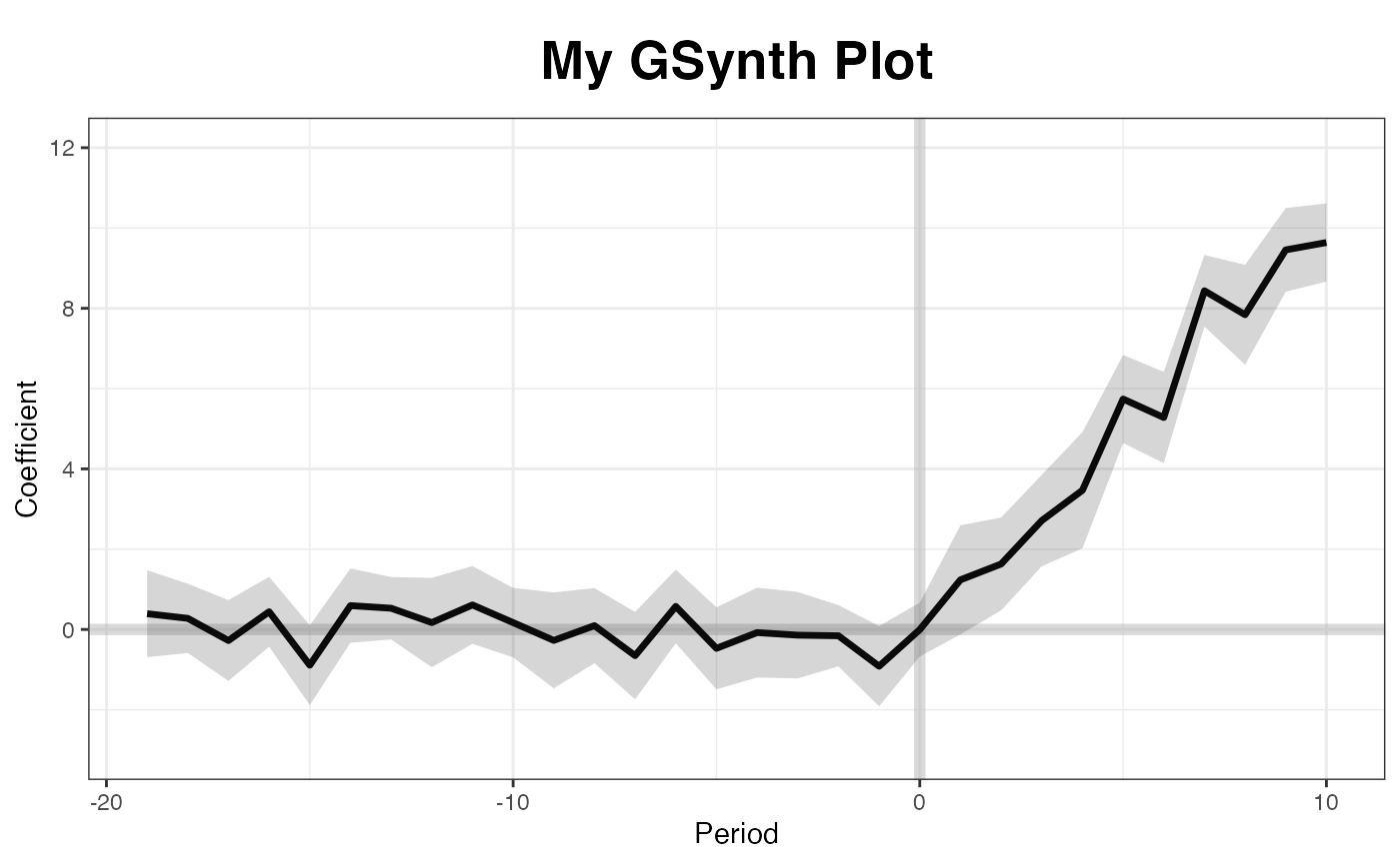
By default, the plot function produce a “gap” plot –
as if we type plot(out, type = "gap") – which visualize the
estimated ATT by period. For your reference, the true effects in
simdata go from 1 to 10 (plus some white noise) from period
21 to 30. You can save the graph, a ggplot2 object, by
directing print to an object name.
plot(out) # by default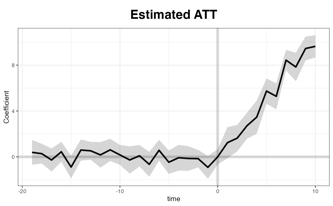
A default ggplot2 theme is available, too:
plot(out, theme.bw = FALSE) 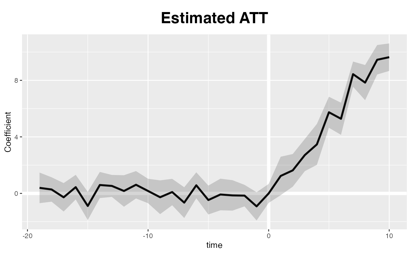
Users can adjust xlim and ylim, and supply
the plot title and titles for the two axes.
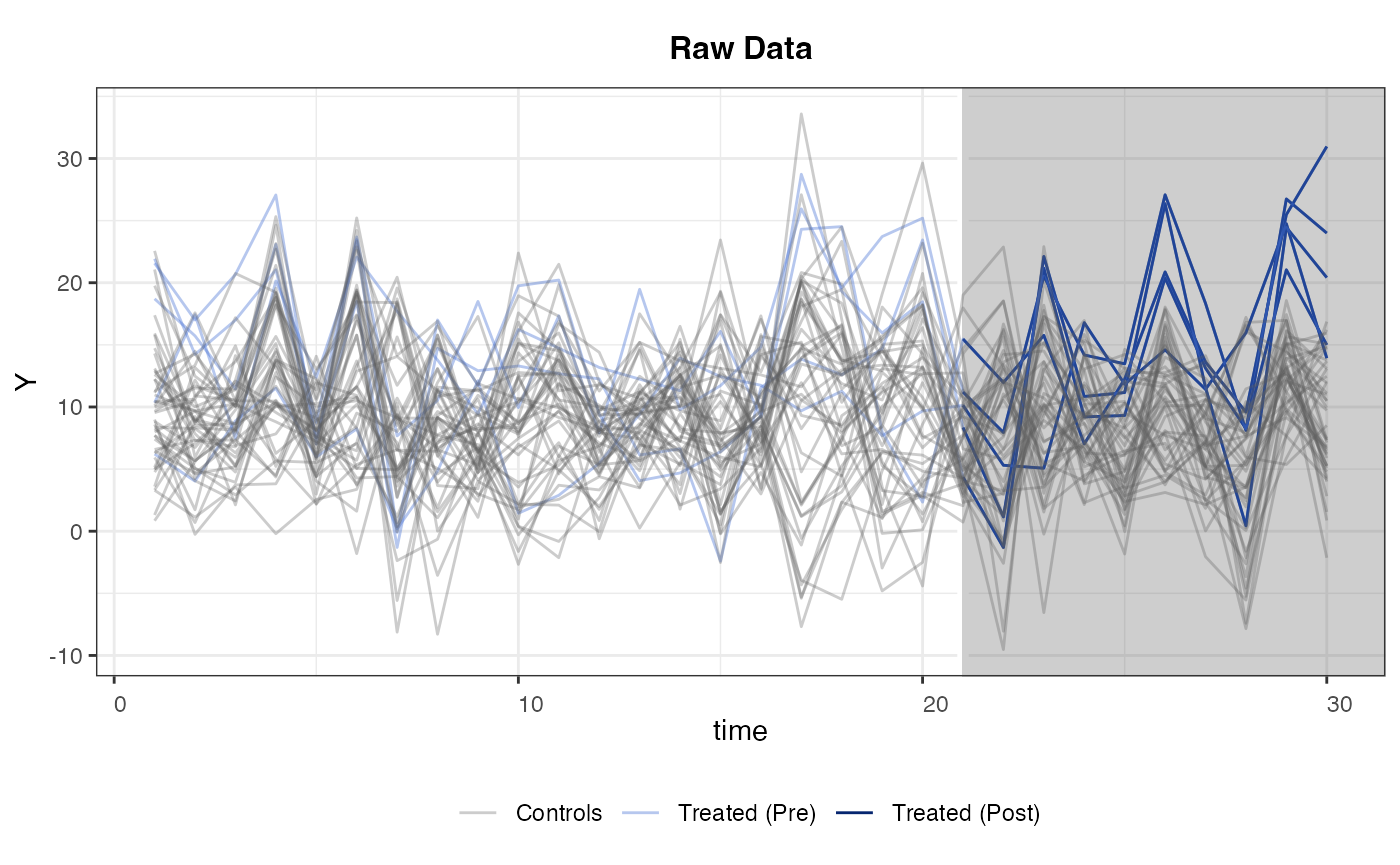
The other four type options include "raw",
which plots the raw data (outcome) variable as
panelview does; "counterfactual" (or
"ct" for short), which plots the estimated
counterfactual(s); and "factors" and
"loadings", which plot estimated factors and loadings,
respectively. The next figure is a raw plot with a black-and-white
theme. The treated (pre- and post-treatment) and control units are
painted with different colors.
plot(out, type = "raw")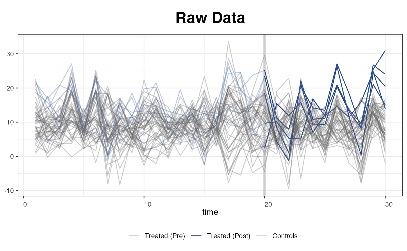
We can set the axes limits, remove the legend and title, for example, by typing (figure not shown):
We use the following line of command to plot the estimated
counterfactual. raw = "none" (the default option) means
that we do not include the raw data in this figure:
plot(out, type = "counterfactual", raw = "none", main="")
One can use shade.post to control the shading in the
post-treatment period
plot(out, type = "ct", raw = "none", main = "",
     shade.post = FALSE)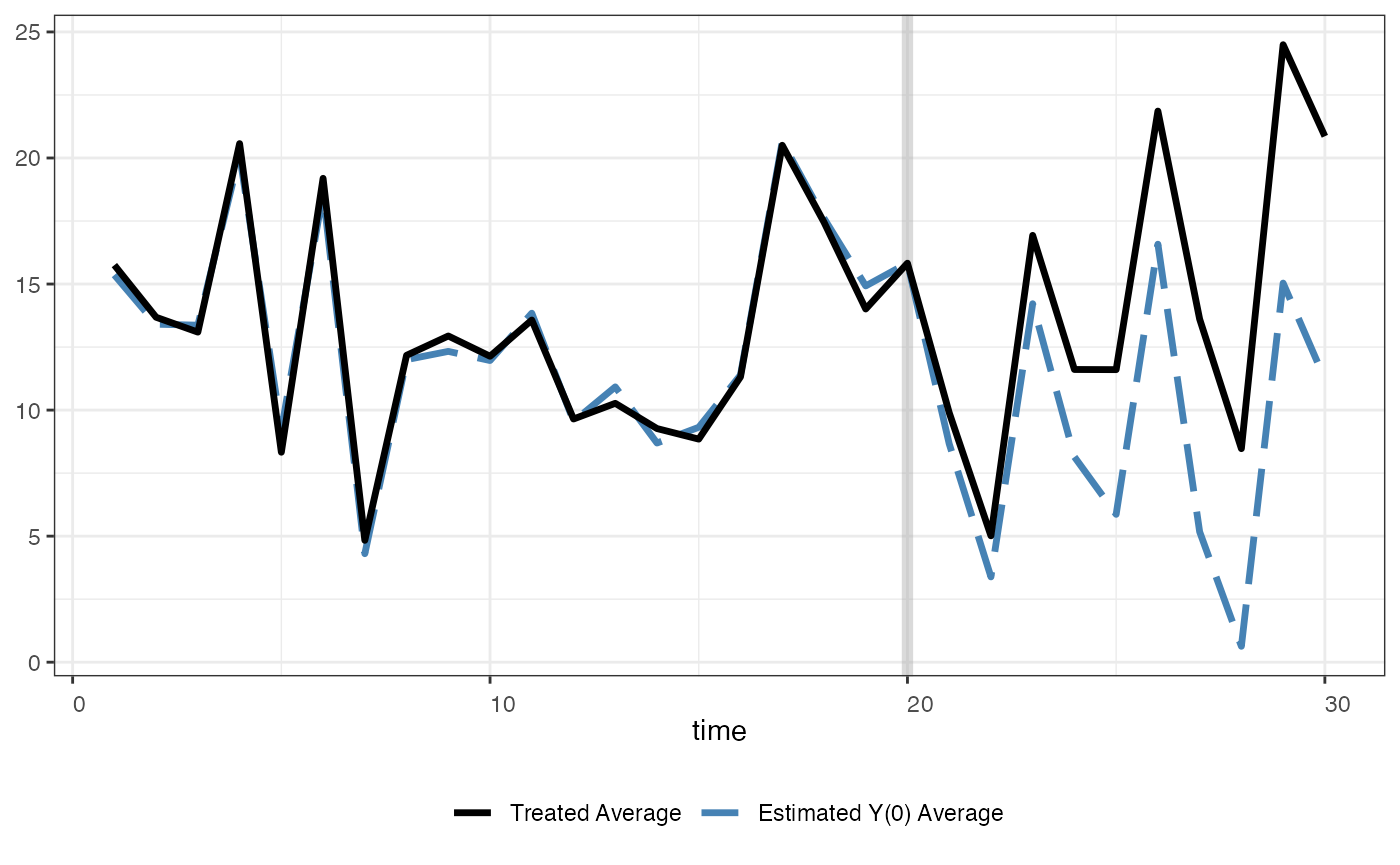
We can also add two 5 to 95% quantile bands of the treated and control outcomes as references to make sure the estimated counterfactuals are not results of severe extrapolations.
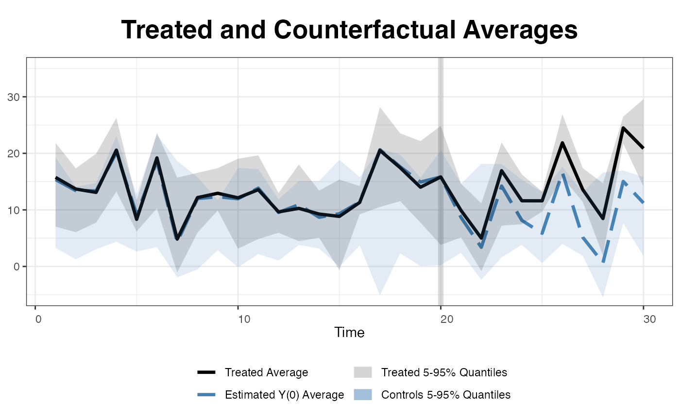
… or simply plot all the raw data (for the outcome variable).
plot(out, type = "counterfactual", raw = "all")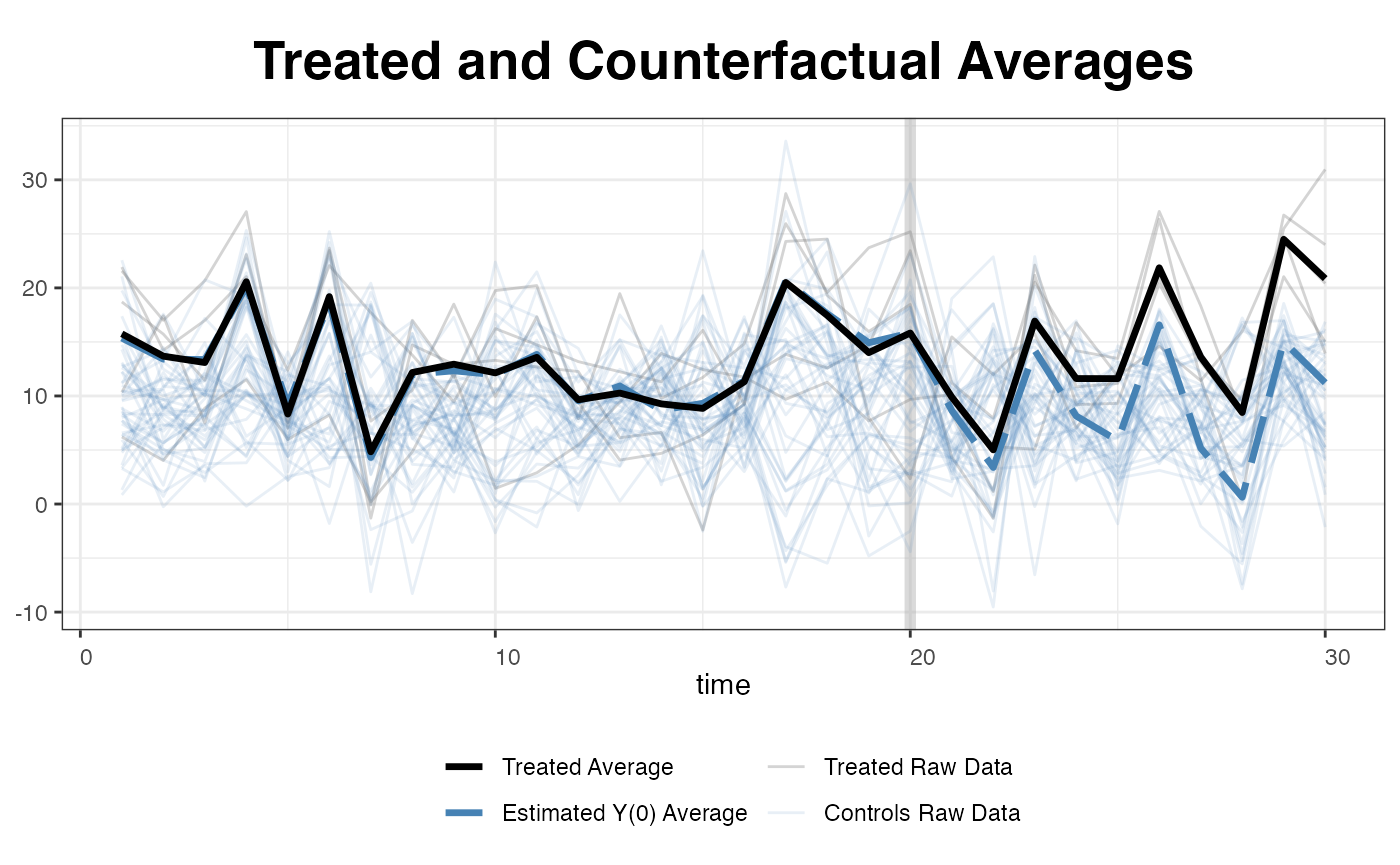
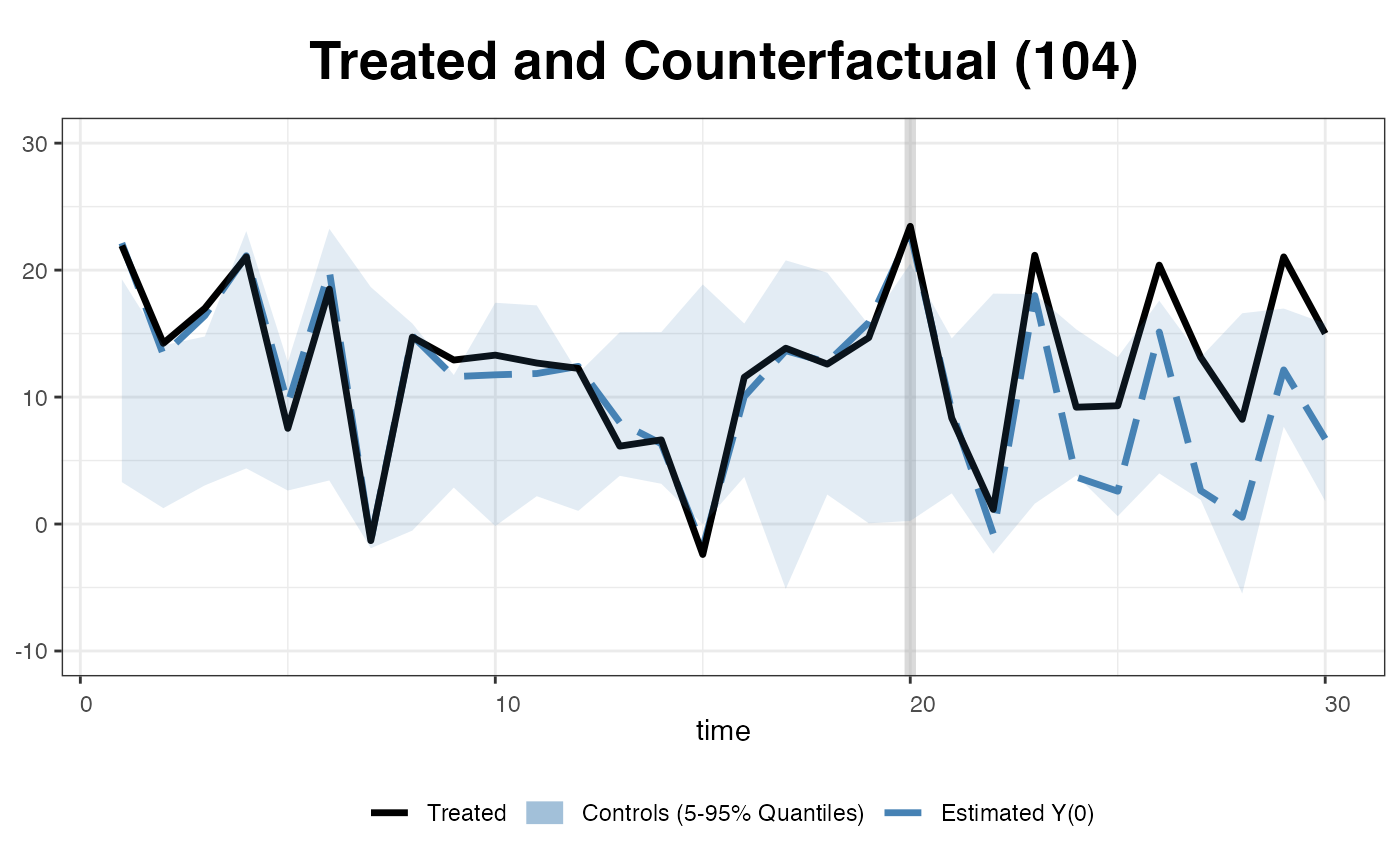
One can also visualize the estimated counterfactual for each treated unit to evaluate the quality of model fit.
plot(out, type = "counterfactual", id = 102)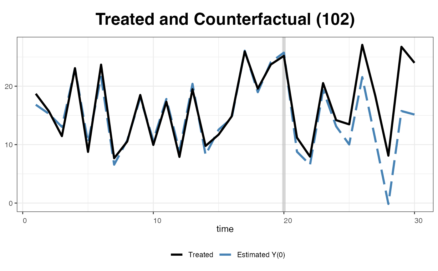
We can add the reference band, a 5 to 95% quantile band the control outcomes.
… or replaced the band with the raw data of the control outcomes.
plot(out, type = "counterfactual", id = 105,
     raw = "all", legendOff = TRUE)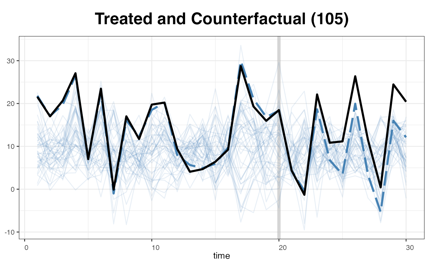
The next two figures plot the estimated factors and factor loadings, respectively.
plot(out, type = "factors", xlab = "Time")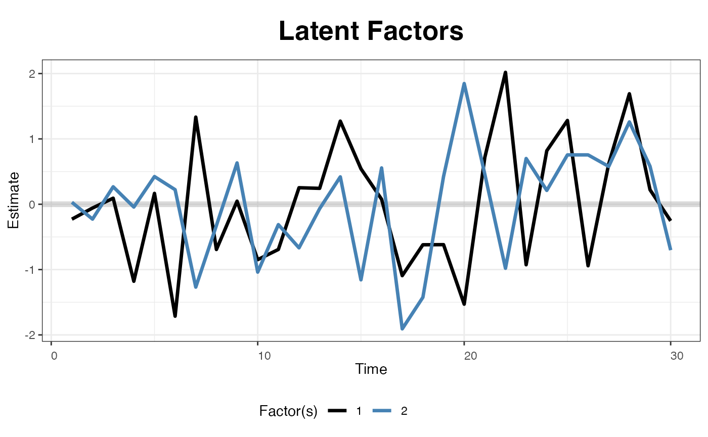
plot(out, type = "loadings")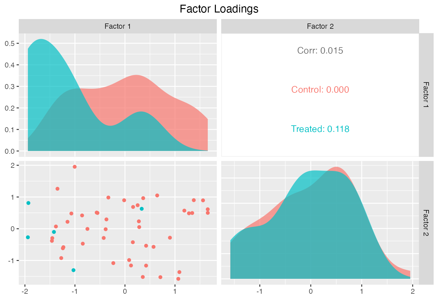
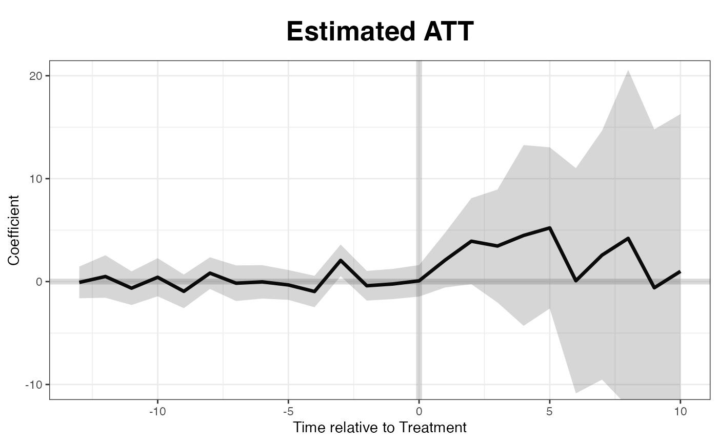
EM method
The EM algorithm proposed by Gobillon and
Magnac (2016) takes advantage of the treatment group information
in the pre-treatment period. We implement this method. The estimation
takes more time, but the results are very similar to that from the
original method – the coefficients will be slightly more precisely
estimated. Only nonparametric or jackknife
inference is allowed when EM is turned on.
system.time(
out <- gsynth(Y ~ D + X1 + X2, data = simdata,
              index = c("id","time"), EM = TRUE,
              force = "two-way", inference = "nonparametric",
              se = TRUE, nboots = 500, r = c(0, 5),
              CV = TRUE, parallel = TRUE, cores = 10)
)
#> Parallel computing ...
#> Cross-validating ...
#> Criterion: Mean Squared Prediction Error
#> Interactive fixed effects model...
#> r = 0; sigma2 = 1.87052; IC = 1.03286; PC = 1.76603; MSPE = 2.17139
#> r = 1; sigma2 = 1.50792; IC = 1.20393; PC = 1.92888; MSPE = 1.90781
#> r = 2; sigma2 = 0.99174; IC = 1.16142; PC = 1.60223; MSPE = 1.33352
#> *
#> r = 3; sigma2 = 0.93513; IC = 1.46912; PC = 1.82665; MSPE = 1.54731
#> r = 4; sigma2 = 0.88552; IC = 1.77104; PC = 2.03006; MSPE = 2.50934
#> r = 5; sigma2 = 0.84141; IC = 2.06634; PC = 2.21549; MSPE = 2.84625
#>
#>  r* = 2
#> Can't calculate the F statistic because of insufficient treated units.
#>    user  system elapsed
#>   1.495   0.171   7.118
plot(out, main = "Estimated ATT (EM)")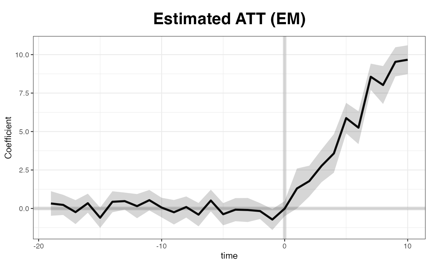
Matrix completion
We implement the matrix completion method proposed by Athey et al. (2021) by setting
estimator = "mc" (the default is "ife", which
represents the interactive fixed effects model). Only
nonparametric or jackknife inference is
allowed.
Matrix completion uses a different regularization scheme and takes
advantage of the treatment group information in the pre-treatment
period. The option lambda controls the tuning parameter. If
it is left blank, a sequence of candidate lambdas will be
generated and tested sequentially. Users can set the length of candidate
list by setting, for example, nlambda = 10. The option
lambda can also receive a user-specified sequence as
candidate lambdas. A built in cross-validation procedure
will select the optimal hyper parameter when a single
lambda is given. Users can specify the number of folds in
cross-validation using the option k
(e.g. k = 5).
system.time(
out <- gsynth(Y ~ D + X1 + X2, data = simdata,
              estimator = "mc", index = c("id","time"),
              se = TRUE, nboots = 500, r = c(0, 5),
              CV = TRUE, force = "two-way",
              parallel = TRUE, cores = 10,
              inference = "nonparametric")
)
#> Parallel computing ...
#> Cross-validating ...
#> Criterion: Mean Squared Prediction Error
#> Matrix completion method...
#> lambda.norm = 1.00000; MSPE = 2.39699; MSPTATT = 0.69437; MSE = 1.97846
#> lambda.norm = 0.42170; MSPE = 1.86827; MSPTATT = 0.31226; MSE = 1.02780
#> *
#> lambda.norm = 0.17783; MSPE = 2.05353; MSPTATT = 0.09063; MSE = 0.31477
#> lambda.norm = 0.07499; MSPE = 2.23786; MSPTATT = 0.01738; MSE = 0.06379
#> lambda.norm = 0.03162; MSPE = 2.26792; MSPTATT = 0.00308; MSE = 0.01170
#>
#>  lambda.norm* = 0.421696503428582
#>
#> Can't calculate the F statistic because of insufficient treated units.
#>    user  system elapsed
#>   1.087   0.169   6.344
plot(out, main = "Estimated ATT (MC)")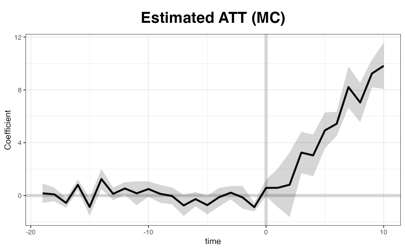
Staggered DID
The second example investigates the effect of Election-Day Registration (EDR) reforms on voter turnout in the United States. Note that the treatment kicks in at different times.
data(gsynth)
names(turnout)
#> [1] "abb"            "year"           "turnout"        "policy_edr"
#> [5] "policy_mail_in" "policy_motor"
Data structure
First, we take a look at the data structure. The following figure shows that (1) we have a balanced panel with 9 treated units and (2) the treatment starts at different time periods.
panelview(turnout ~ policy_edr, data = turnout,
          index = c("abb","year"), pre.post = TRUE,
by.timing = TRUE) 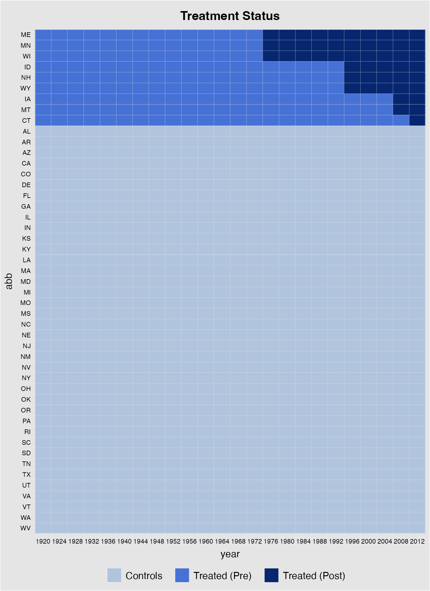
panelview can also visualize the outcome variable by group (change in treatment status)
panelview(turnout ~ policy_edr, data = turnout,
          index = c("abb","year"), type = "outcome",
          main = "EDR Reform and Turnout",
          by.group = TRUE)
#> Warning in panelview(turnout ~ policy_edr, data = turnout, index = c("abb", :
#> option "by.cohort" is not allowed with "by.group = TRUE" or "by.group.side =
#> TRUE". Ignored.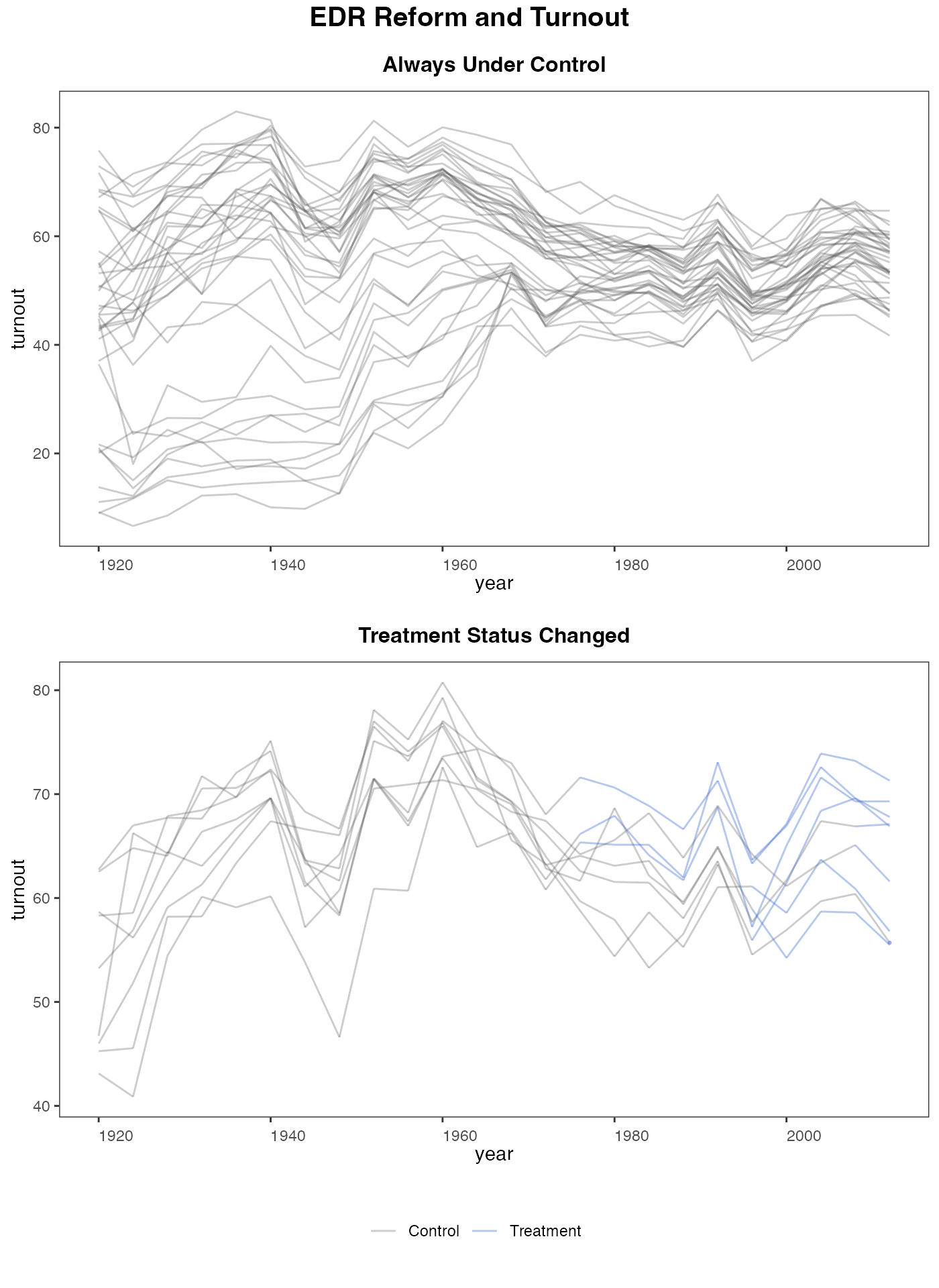
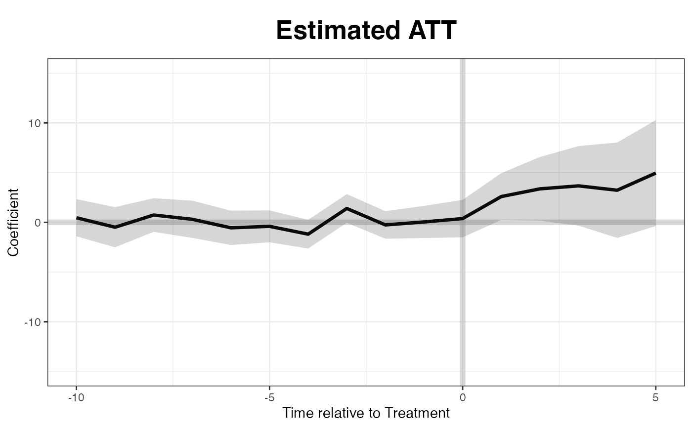
Estimation w/o factors
When no factor is assumed, the estimates are close to what we obtain from difference-in-differences:
out0 <- gsynth(turnout ~ policy_edr + policy_mail_in + policy_motor,
               data = turnout, index = c("abb","year"),
               se = TRUE, inference = "parametric",
               r = 0, CV = FALSE, force = "two-way",
               nboots = 1000, seed = 02139)
#> Parallel computing ...
#> Parametric Bootstrap
#> Simulating errors ...
#> Can't calculate the F statistic because of insufficient treated units.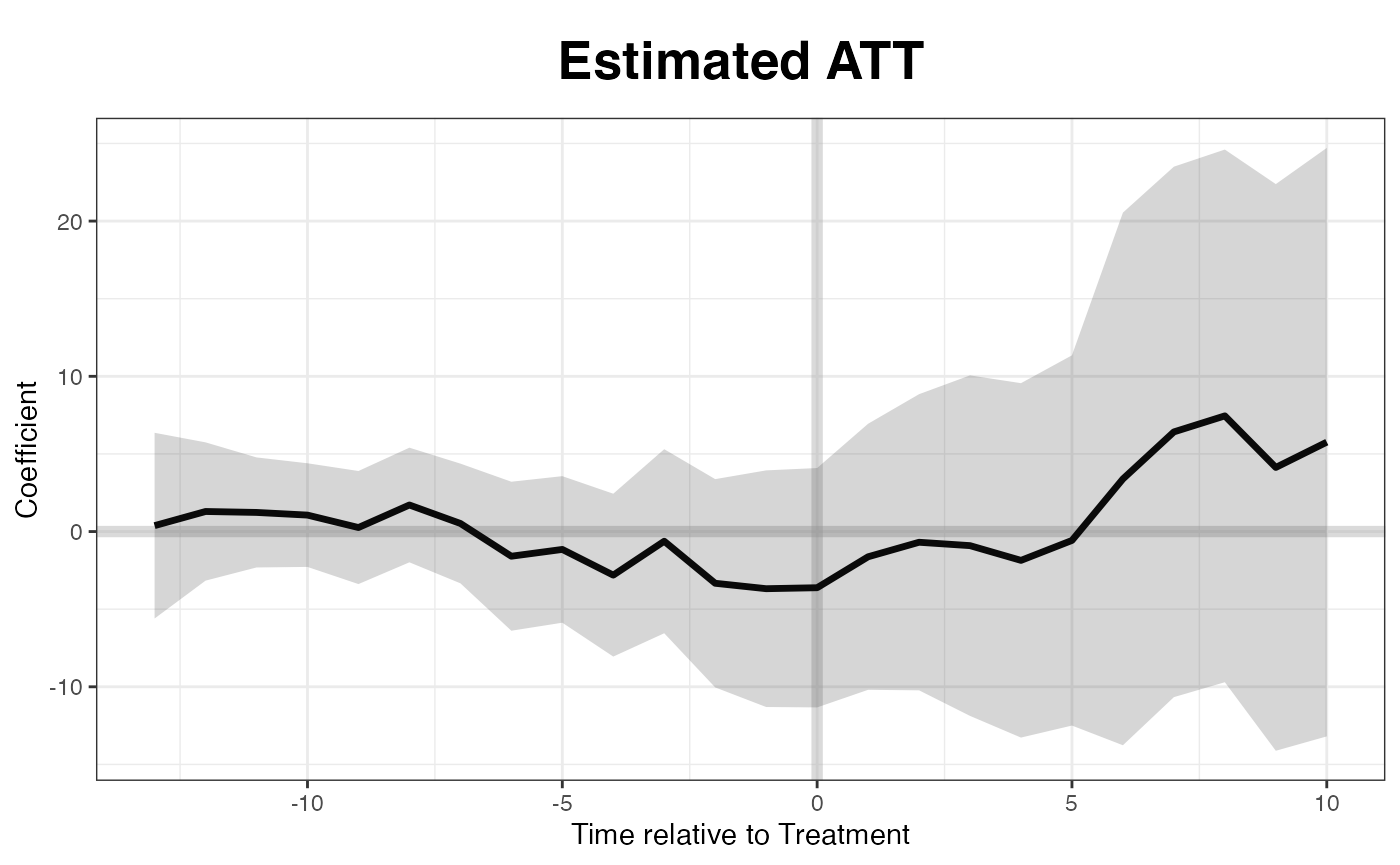
Estimation w/ factors
Now we allow the algorithm to find the “correct” number of factors that predicts the pre-treatment data the best:
out <- gsynth(turnout ~ policy_edr + policy_mail_in + policy_motor,
              data = turnout,  index = c("abb","year"),
              se = TRUE, inference = "parametric",
              r = c(0, 5), CV = TRUE, force = "two-way",
              nboots = 1000, seed = 02139)
#> Parallel computing ...
#> Cross-validating ...
#> Criterion: Mean Squared Prediction Error
#> Interactive fixed effects model...
#> Cross-validating ...
#> r = 0; sigma2 = 77.99366; IC = 4.82744; PC = 72.60594; MSPE = 22.13889
#> r = 1; sigma2 = 13.65239; IC = 3.52566; PC = 21.67581; MSPE = 12.03686
#> r = 2; sigma2 = 8.56312; IC = 3.48518; PC = 19.23841; MSPE = 10.31254
#> *
#> r = 3; sigma2 = 6.40268; IC = 3.60547; PC = 18.61783; MSPE = 11.48390
#> r = 4; sigma2 = 4.74273; IC = 3.70145; PC = 16.93707; MSPE = 16.28613
#> r = 5; sigma2 = 4.02488; IC = 3.91847; PC = 17.05226; MSPE = 15.78683
#>
#>  r* = 2
#>
#> Parametric Bootstrap
#> Simulating errors ...
#> Can't calculate the F statistic because of insufficient treated units.
Implied weights
out$wgt.implied
()
stores the implied weights of all control units for each treated unit.
Different from the synthetic control method, the weights can be both
positive and negative. Below we show the control unit weights for
Wisconsin.
dim(out$wgt.implied)
#> [1] 38  9
sort(out$wgt.implied[,8])
#>  [1] -0.420446734 -0.359404870 -0.358899140 -0.323621805 -0.275363471
#>  [6] -0.222140041 -0.214909889 -0.197804828 -0.185884567 -0.162290117
#> [11] -0.151519318 -0.148094608 -0.127000746 -0.064591440 -0.057043363
#> [16] -0.038932843 -0.001453018  0.010929464  0.029620626  0.049794411
#> [21]  0.073077120  0.079864605  0.090892631  0.091876103  0.093457125
#> [26]  0.104411283  0.133990028  0.158671615  0.159121640  0.181418421
#> [31]  0.182877791  0.221808796  0.226279566  0.250193486  0.278783695
#> [36]  0.280519519  0.295315162  0.316497707
Plot results
The missing data plot can also be produced after the estimation is performed. In addition, plot allows users to changes axes labels and the graph title (figure not shown).
plot(out, type = "missing", main = "Treatment Status",
     xlab = "Year", ylab = "State")
The following line of code produces the “gap” plot:
If we want to know the treatment effect on a specific state, such as
Wisconsin, we can specify the id option:
plot(out, type = "gap", id = "WI", main = "Wisconsin")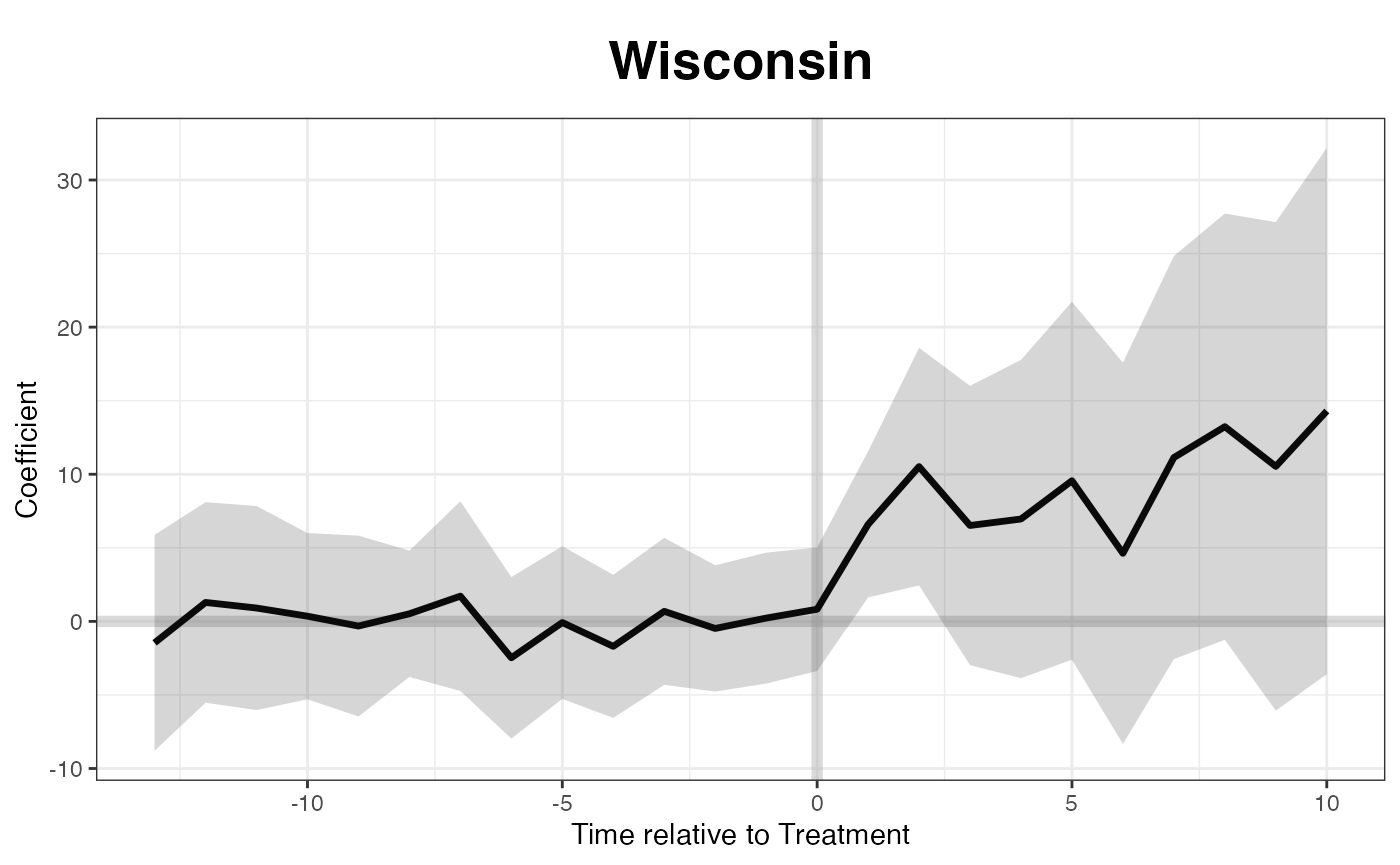
Plotting the raw turnout data:
plot(out, type = "raw", xlab = "Year", ylab = "Turnout")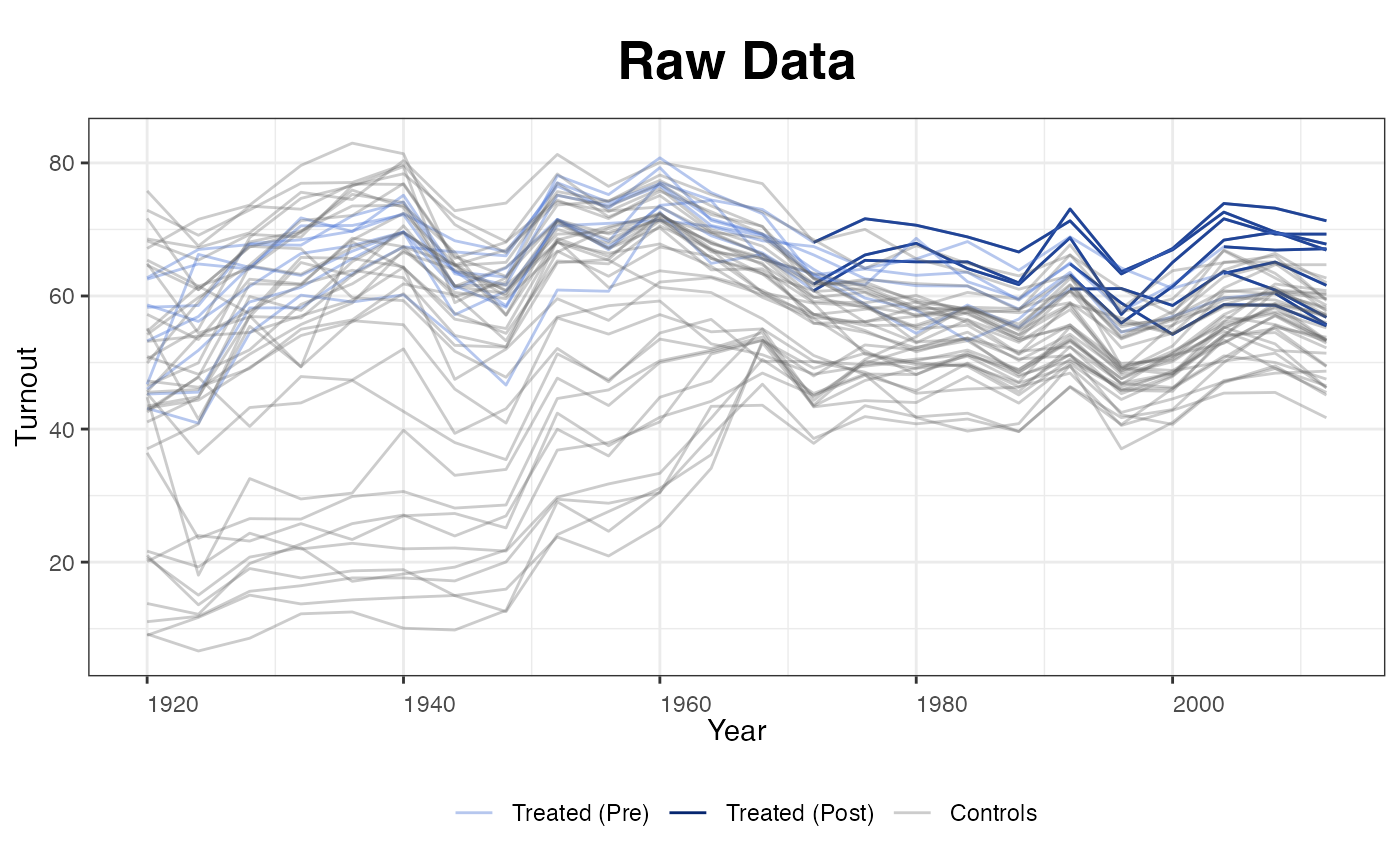
Plotting the estimated average counterfactual. Since EDR reforms kick
in at different times, the algorithm realign the x-axis based on the
timing of the treatment. raw = all shows the realigned
outcomes of the treated units.
plot(out, type = "counterfactual", raw = "all")
#> Warning: Removed 73 rows containing missing values or values outside the scale range
#> (`geom_line()`).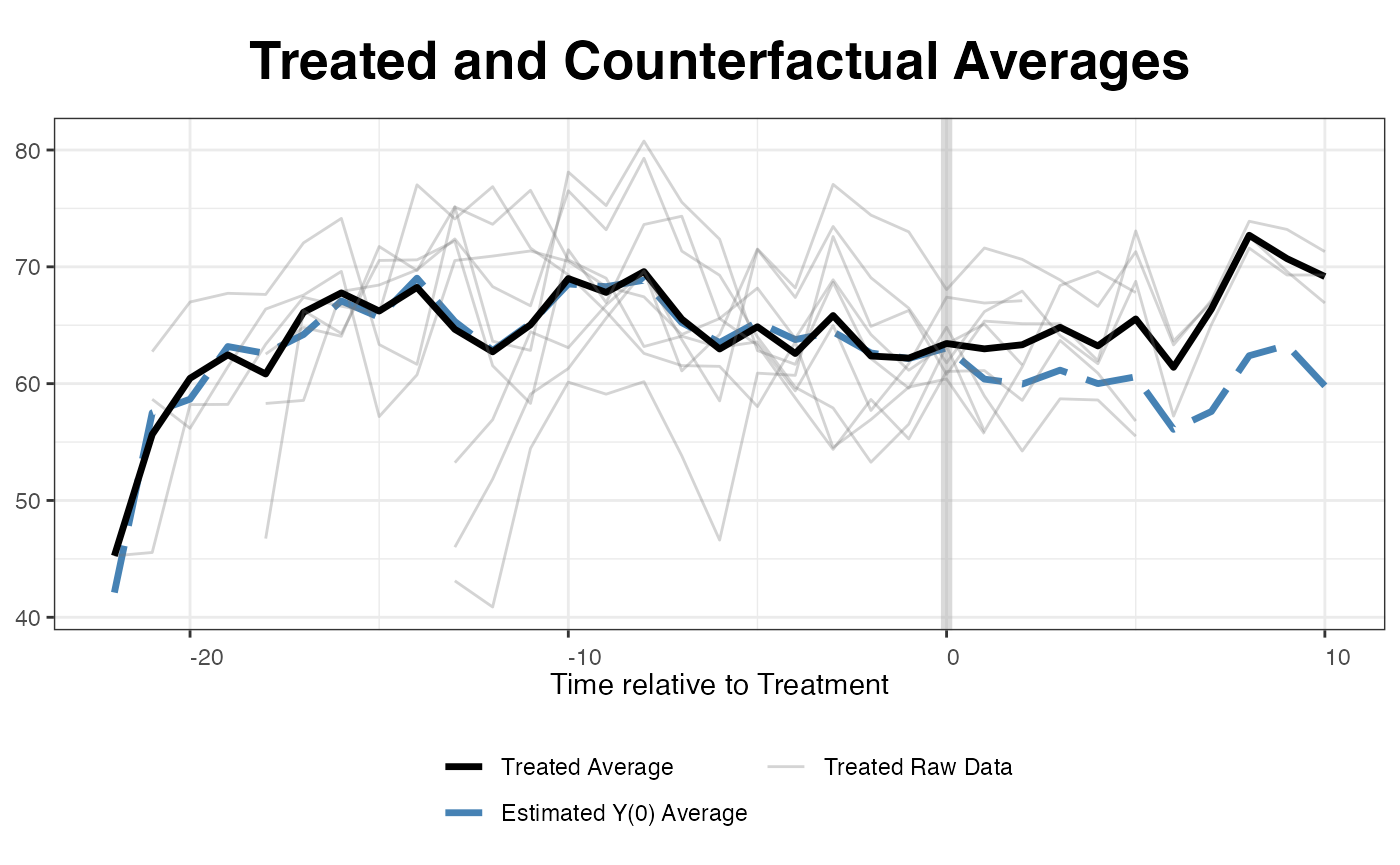
We can plot estimated counterfactuals for each treated unit:
plot(out, type="counterfactual", id = "CT")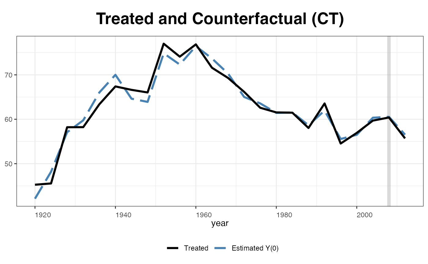
plot(out, type = "counterfactual", id = "WY",
     raw = "all", legendOff = TRUE)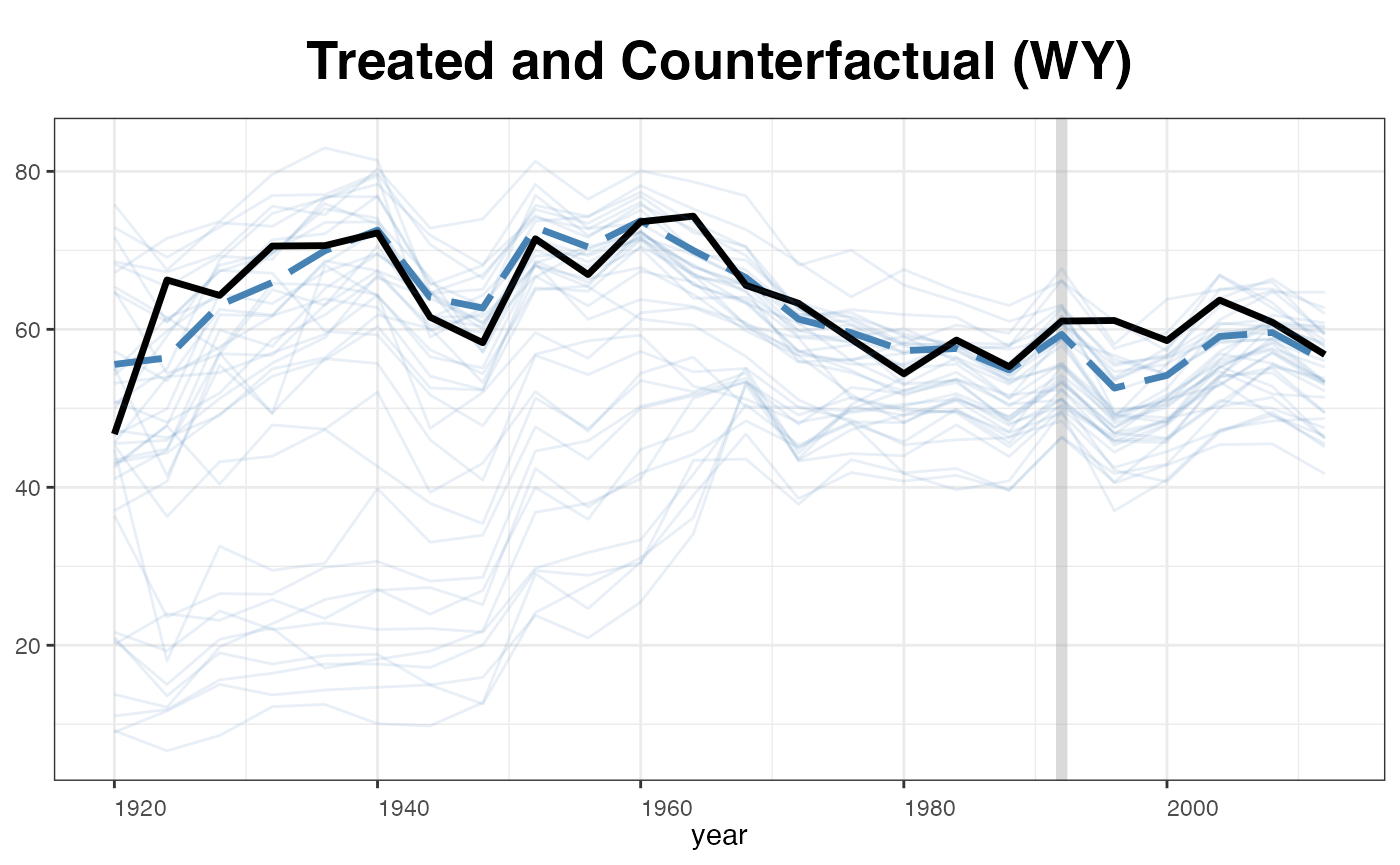
plot(out, type = "counterfactual", id = "WI",
     raw = "none", shade.post = FALSE, ylim = c(0,100),
     legend.labs = c("Wisconsin Actual","Wisconsin Counterfactural"))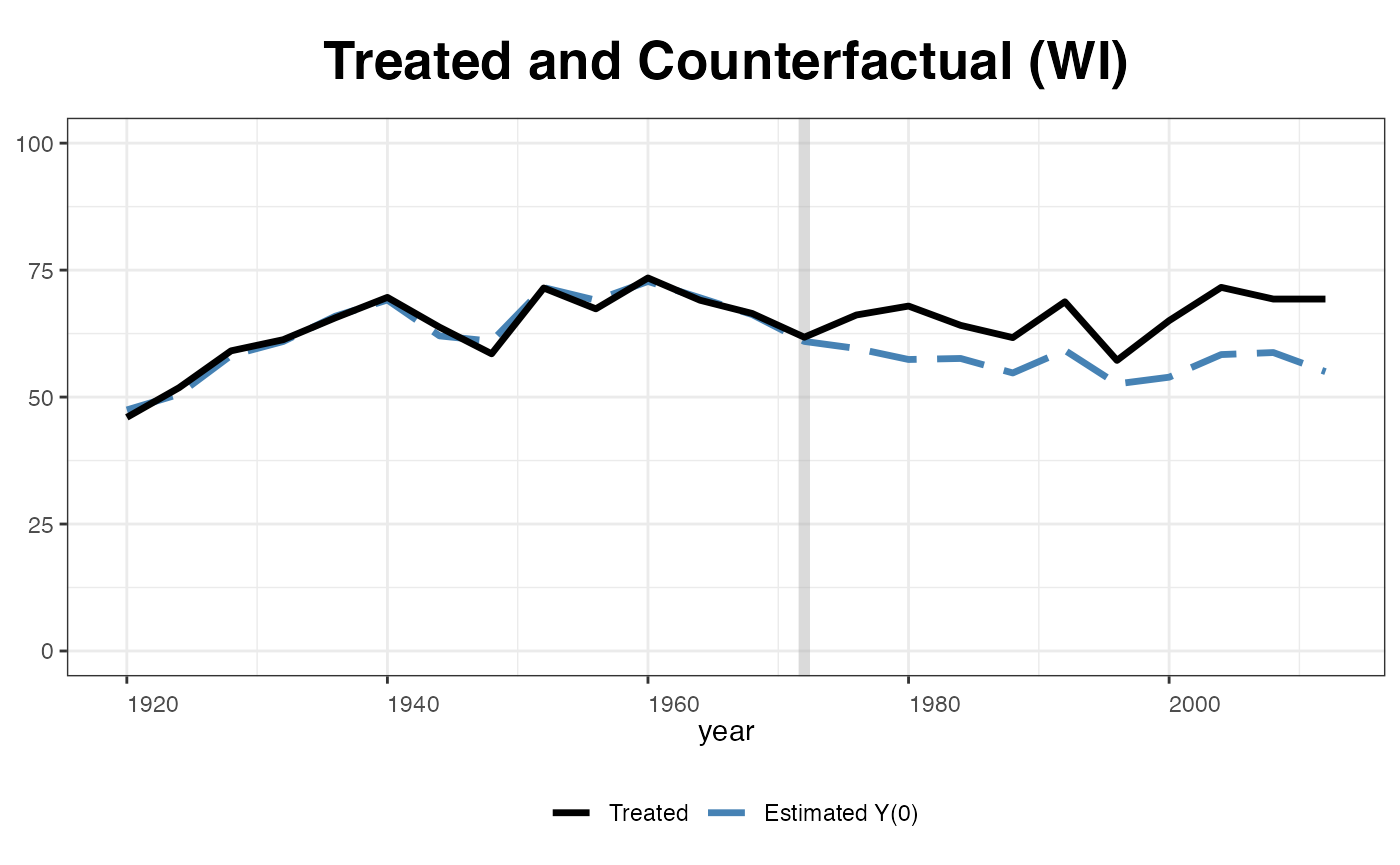
Estimated factors and factor loadings::
plot(out, type = "factors", xlab="Year")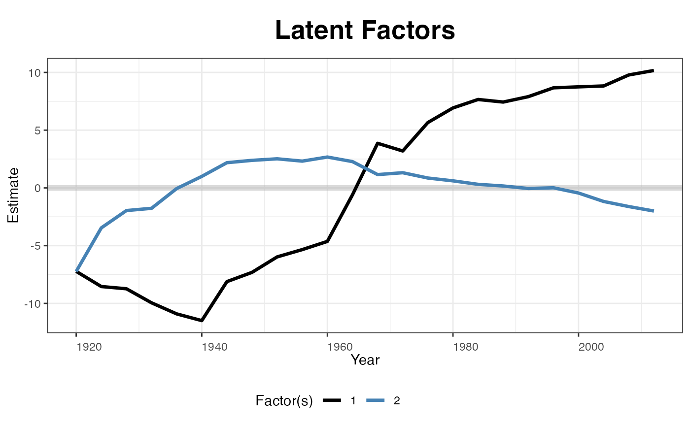
plot(out, type = "loadings")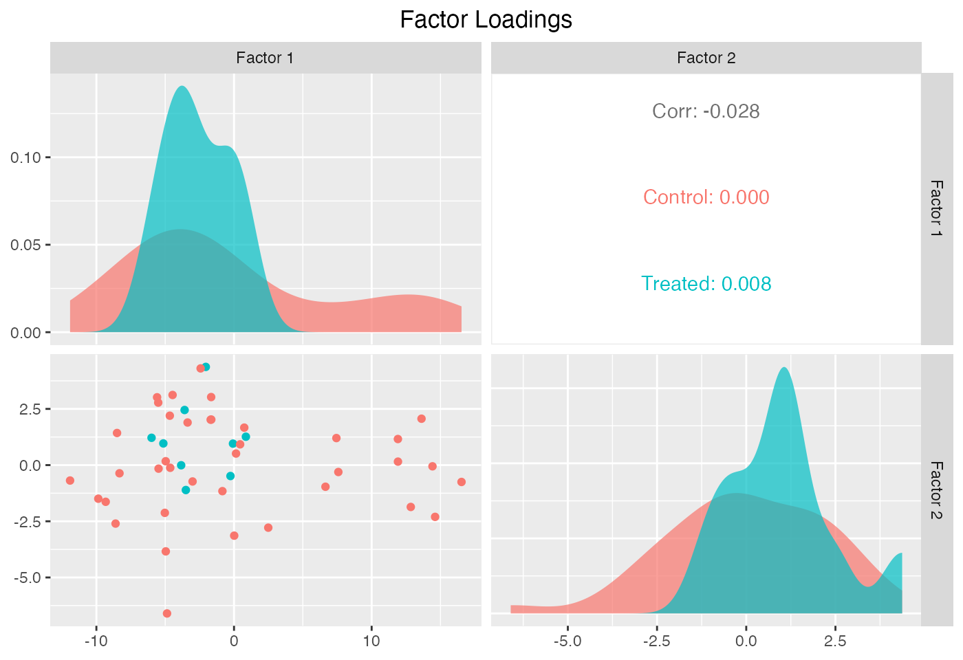
Unbalanced panels
gsynth can accommodate unbalanced panels. To illustrate how it works, we randomly remove 50 observations as well as the first 15 observations of Wyoming from the turnout dataset and then re-estimate the model:
set.seed(123456)
turnout.ub <- turnout[-c(which(turnout$abb=="WY")[1:15],
                         sample(1:nrow(turnout),50,replace=FALSE)),]
Again, before running any regressions, we first plot the data structure and visualize missing values. In the following plot, white cells represent missing values.
panelview(turnout ~ policy_edr + policy_mail_in + policy_motor,
          data = turnout.ub,  index = c("abb","year"),
pre.post = TRUE) 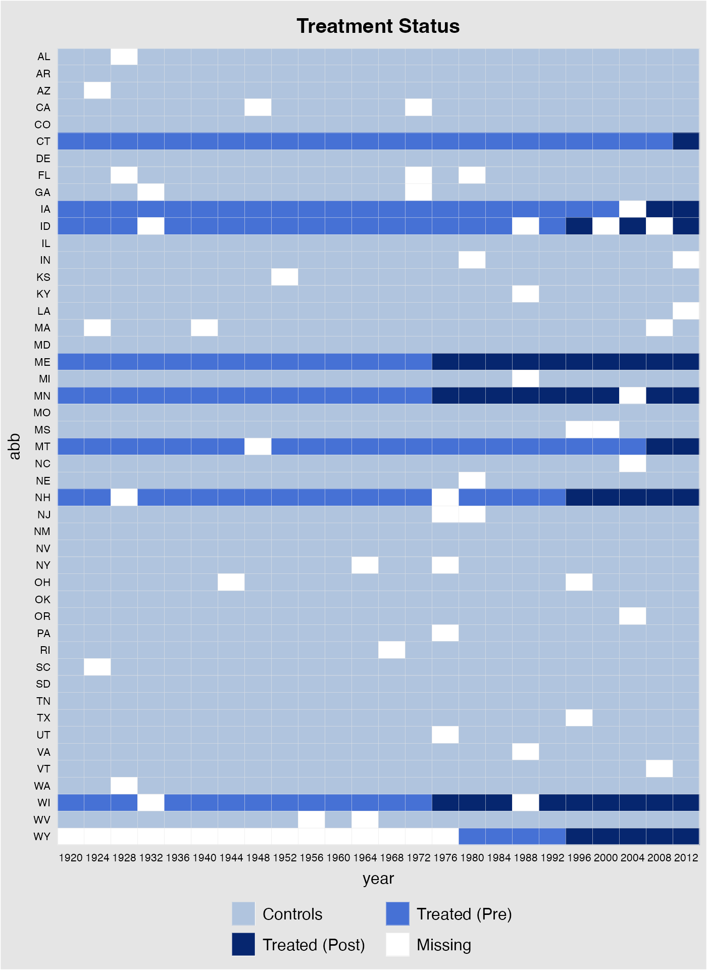
Estimation
out <- gsynth(turnout ~ policy_edr + policy_mail_in + policy_motor,
              data = turnout.ub,  index = c("abb","year"),
              se = TRUE, inference = "parametric",
              r = c(0, 5), CV = TRUE, force = "two-way",
              parallel = TRUE, min.T0 = 8,
              nboots = 1000, seed = 02139)
#> For identification purposes, units whose number of untreated periods <8 are dropped automatically.
#> Parallel computing ...
#> Cross-validating ...
#> Criterion: Mean Squared Prediction Error
#> Interactive fixed effects model...
#> Cross-validating ...
#> r = 0; sigma2 = 78.53850; IC = 4.85229; PC = 72.87077; MSPE = 19.00413
#> r = 1; sigma2 = 13.71115; IC = 3.56457; PC = 22.12908; MSPE = 11.91054
#> r = 2; sigma2 = 8.64454; IC = 3.54545; PC = 19.90277; MSPE = 7.61167
#> r = 3; sigma2 = 6.52720; IC = 3.69114; PC = 19.53620; MSPE = 7.56166
#> *
#> r = 4; sigma2 = 4.83105; IC = 3.80135; PC = 17.80738; MSPE = 15.96018
#> r = 5; sigma2 = 4.16136; IC = 4.04774; PC = 18.23222; MSPE = 15.64924
#>
#>  r* = 3
#>
#> Parametric Bootstrap
#> Simulating errors ...
#> Can't calculate the F statistic because of insufficient treated units.
Plot results
The missing plot visualizes the data being used in the
regression (similar to that from turning on quick_missing
in the main function). It is different from the plot generated from
panelview in that observations for Wyoming are now
represented by gray cells with red dots to indicate that they are
removed from the sample because of insufficient number of pre-treatment
periods. The missing data matrix can also be retrieved from
out$obs.missing, in which 0, 1, 2, 3 4 represent missing
values, control observations, treated (pre-treatment) observations,
treated (post-treatment) observations, and treated observations removed
from the sample, respectively.
plot(out, type = "missing")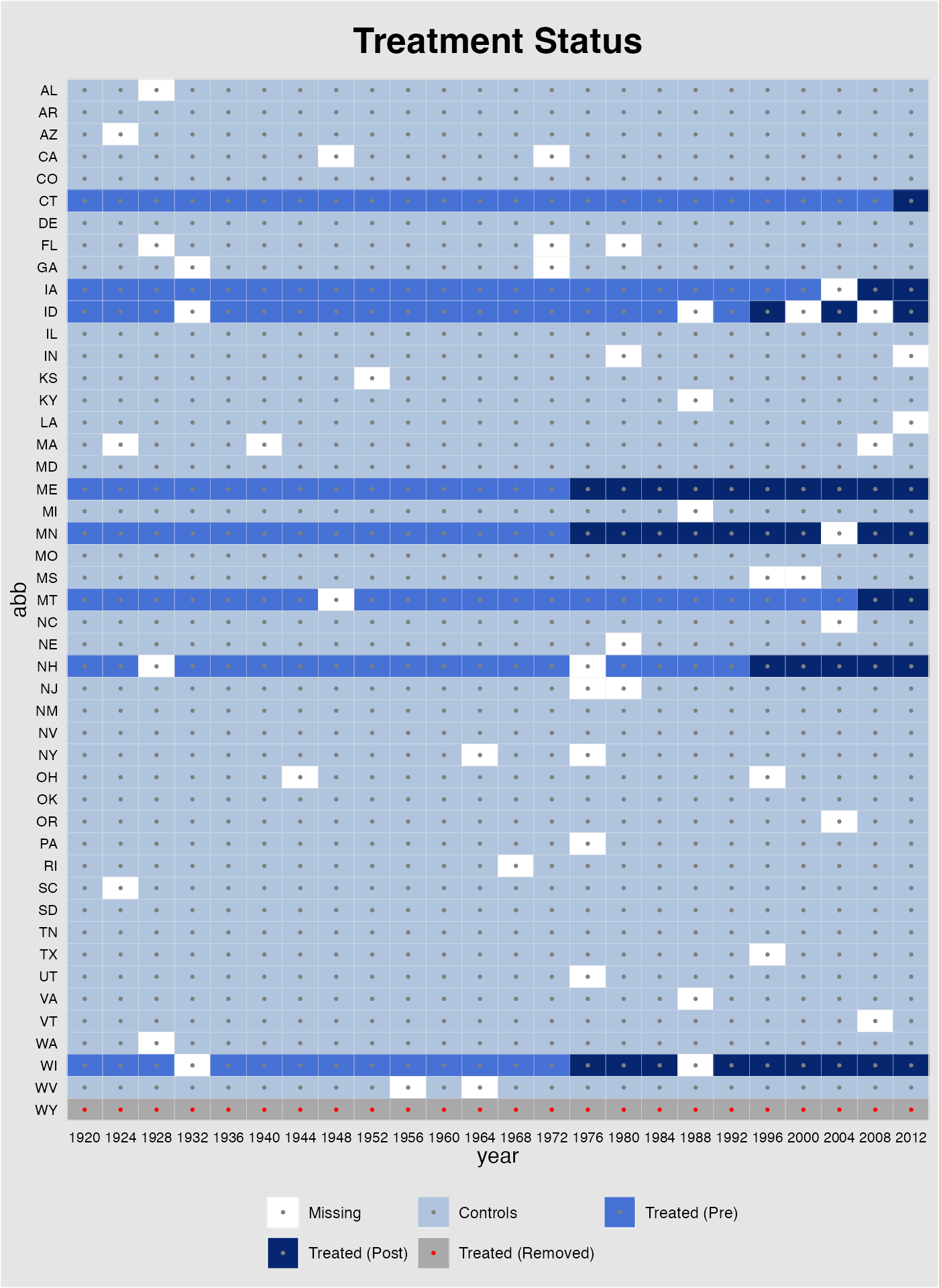
Like in panelview, users can plot part of all units
by specifying id and adjust labels on x-axis when the the
magnitude of data is too large.
plot(out, type = "missing", xlab = "Year", ylab = "State",
     main = "Treatment Status", id = out$id.tr,
     xlim = c(1920,2012),  axis.adjust=TRUE)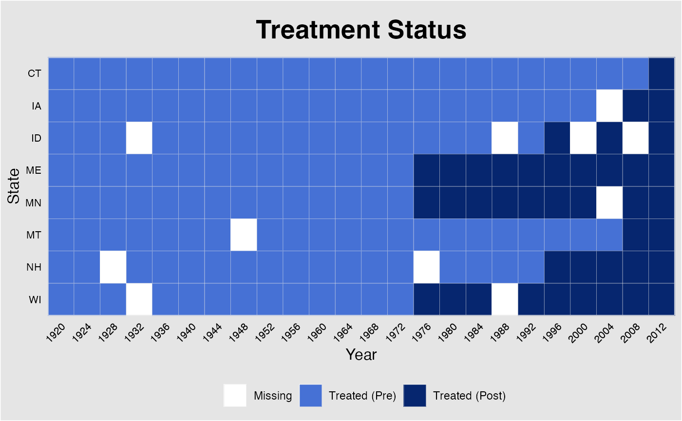
We re-produce the “gap” plot with the unbalanced panel:
Matrix completion
Finally, we re-estimate the model using the matrix completion method:
out.mc <- gsynth(turnout ~ policy_edr + policy_mail_in + policy_motor,
                 min.T0 = 8, data = turnout.ub,
                 index = c("abb","year"), estimator = "mc",
                 se = TRUE, nboots = 1000, seed = 02139)
#> For identification purposes, units whose number of untreated periods <8 are dropped automatically.
#> Parallel computing ...
#> Cross-validating ...
#> Criterion: Mean Squared Prediction Error
#> Matrix completion method...
#> lambda.norm = 1.00000; MSPE = 110.44231; MSPTATT = 37.48243; MSE = 253.92696
#> lambda.norm = 0.42170; MSPE = 61.05209; MSPTATT = 35.03747; MSE = 226.25753
#> lambda.norm = 0.17783; MSPE = 30.76102; MSPTATT = 33.44296; MSE = 206.27740
#> lambda.norm = 0.07499; MSPE = 20.75095; MSPTATT = 32.78161; MSE = 198.55570
#> *
#> lambda.norm = 0.03162; MSPE = 22.60698; MSPTATT = 32.05467; MSE = 196.15491
#> lambda.norm = 0.01334; MSPE = 40.48386; MSPTATT = 31.68165; MSE = 197.29681
#> lambda.norm = 0.00562; MSPE = 83.66856; MSPTATT = 32.28561; MSE = 203.16360
#>
#>  lambda.norm* = 0.0749894209332456
#>
#> Can't calculate the F statistic because of insufficient treated units.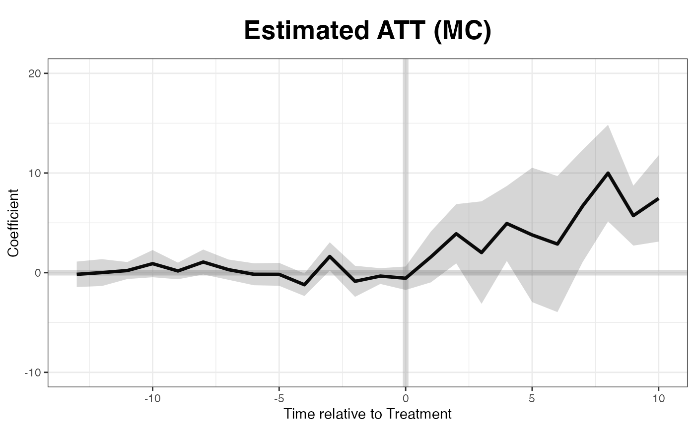
Additional Notes
Running gsynth with unbalanced panels will take significantly more time than with balanced panels (the magnitude is often 100:1 or even higher). This is because the EM algorithm that fills in missing values (also written in C++) runs many more loops. This means users can often significantly reduce run-time by removing some units or time periods that have many missing values. Knowing the data structure before running any regressions always helps!
Similarly, adding covariates will significantly slow down the algorithm because the IFE/MC model will take more time to converge.
Set
min.T0to a positive number helps. The algorithm will automatically discard treated units that have too few pre-treatment periods. A bigger reduces bias in the causal estimates and the chances of severe extrapolation. If users run cross-validation to select the number of factors,min.T0needs to be equal to or greater than (r.max+2).