Tutorial
tutorial.RmdIn this tutorial, we illustrate how to use the fect package in R to implement counterfactual estimators and conduct diagnostic tests proposed by Liu, Wang, and Xu (2022). What start with a simulated dataset.
Simulated data
fect ships two datasets. In this demo, we will primarily be using simdata, in which the treatment is allowed to switch on and off. There are 200 units and 35 time periods. We describe its DGP in the paper.
Visualizing the treatment and outcome variables
Before conducting any statistical analysis, we use the panelView package to visualize the treatment and outcome variables in the data. The following line of code plots the treatment status of all units in simdata:
library(panelView)
panelview(Y ~ D, data = simdata, index = c("id","time"),
  axis.lab = "time", xlab = "Time", ylab = "Unit",
  gridOff = TRUE, by.timing = TRUE,
  background = "white", main = "Simulated Data: Treatment Status")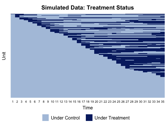
We then take a look at the outcome variable. In the figure below, blue and gray represent treatment and control conditions.
panelview(Y ~ D, data = simdata, index = c("id","time"),
  axis.lab = "time", xlab = "Time", ylab = "Unit",
  theme.bw = TRUE, type = "outcome", main = "Simulated Data: Outcome")
#> Treatment has reversals.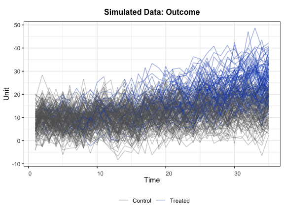
Counterfactual estimators
In the current version of fect, we use three methods
to make counterfactual predictions by specifying the method
option: “fe” (two-way fixed effects, default), “ife” (interactive fixed
effects), and “mc” (matrix completion method). First, we illustrate the
main syntax of fect using the “fe” method.
Two-way Fixed Effects Coutnerfacutal (FEct)
This estimator is also independently proposed by Borusyak, Jaravel, and Spiess (2021) and Gardner (2021), who refer to it as the “imputation method” and “two-stage DID,” respectively.
Estimation. We estimate the average treatment effect
on the treated (ATT) using the following information: the outcome
variable \(Y\), binary treatment
variable \(D\), two observed covariates
\(X_{1}\) and \(X_{2}\), and the unit and time indicators
\(id\) and \(time\), respectively. The first variable on
the right hand side of the formula is the treatment indicator \(D\); the rest of the right-hand-side
variables serve as controls. The index option specifies the
unit and time indicators. The force option (“none”, “unit”,
“time”, and “two-way”) specifies the additive component(s) of the fixed
effects included in the model. The default option is “two-way”
(including both unit and time fixed effects).
out.fect <- fect(Y ~ D + X1 + X2, data = simdata, index = c("id","time"),
  method = "fe", force = "two-way")
Visualization. We can use the plot
function to visualize the estimation results. By default, the
plot function produces a “gap” plot – as if we type
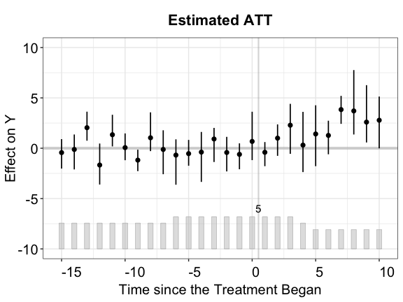
plot(out.fect, type = "gap") — which visualizes the
estimated period-wise ATT (dynamic treatment effects). For your
reference, the true population average effects in
simdata go from 1 to 3 from the 1st to the 10th
post-treatment period.
The bar plot at the bottom of the plot shows the number of treated
units for each time period.The options cex.main,
cex.lab, cex.axis, and cex.text
adjust the font sizes of the title, axis labels, axis numbers, and
in-graph text, respectively.
Users can choose to plot only those periods whose number of
treated observations exceeds a threshold, which is set as a
proportion of the largest number of treated observations in a period
(the default is proportion = 0.3).
plot(out.fect, main = "Estimated ATT (FEct)", ylab = "Effect of D on Y",
  cex.main = 0.8, cex.lab = 0.8, cex.axis = 0.8)
#> Uncertainty estimates not available.
You can then save the graph, a ggplot2 object, by using the ggsave (preferred) function or the print function.
Uncertainty estimates. The algorithm produces
uncertainty estimates when se = TRUE. One can use the
non-parametric bootstrap procedure by setting
vartype = "bootstrap". Note that it only works well when
the number of units is relatively large and many experience the
treatment condition. The number of bootstrap runs is set by
nboots.
Alternatively, users can obtain uncertainty estimates using the
jackknife method by specifying vartype = "jackknife". The
algorithm obtains standard errors by iteratively dropping one unit (the
entire time-series) from the dataset.
Parallel computing will speed up both cross-validation and
uncertainty estimation significantly. When parallel = TRUE
(default) and cores options are omitted, the algorithm will
detect the number of available cores on your computer automatically.
(Warning: it may consume most of your computer’s computational power if
all cores are being used.)
out.fect <- fect(Y ~ D + X1 + X2, data = simdata, index = c("id","time"),
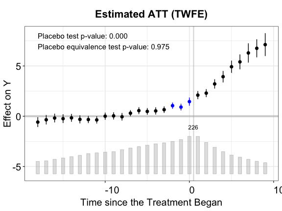
method = "fe", force = "two-way", se = TRUE, parallel = TRUE, nboots = 200)The plot can then visualize the estimated
period-wise ATTs as well as their uncertainty estimates.
stats = "F.p" shows the p-value for the F test of
no-pretrend (more details below).
plot(out.fect, main = "Estimated ATT (FEct)", ylab = "Effect of D on Y",
  cex.main = 0.8, cex.lab = 0.8, cex.axis = 0.8, stats = "F.p")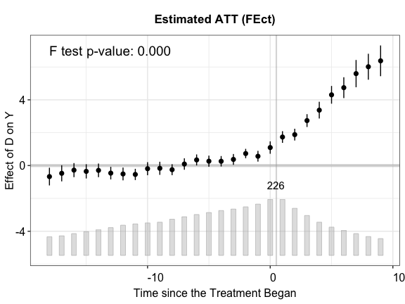
Result summary. Users can use the
print function to take a look at a summary of the
estimation results or retrieve relevant statistics by directly accessing
the fect object. Specifically, est.avg and
est.avg.unit show the ATT averaged over all periods – the
former weights each treated observation equally while the latter weights
each treated unit equally. est.beta reports the
coefficients of the time-varying covariates. est.att
reports the average treatment effect on the treated (ATT) by period.
Treatment effect estimates from each bootstrap run is stored in
eff.boot, an array whose dimension = (#time periods *
#treated * #bootstrap runs).
print(out.fect)
#> Call:
#> fect.formula(formula = Y ~ D + X1 + X2, data = simdata, index = c("id",
#>     "time"), force = "two-way", method = "fe", se = TRUE, nboots = 200,
#>     parallel = TRUE)
#>
#> ATT:
#>                             ATT   S.E. CI.lower CI.upper p.value
#> Tr obs equally weighted   5.121 0.3226    4.488    5.753       0
#> Tr units equally weighted 3.622 0.2611    3.110    4.133       0
#>
#> Covariates:
#>     Coef    S.E. CI.lower CI.upper p.value
#> X1 1.015 0.03666   0.9433    1.087       0
#> X2 2.937 0.03441   2.8695    3.004       0
To save space, results are not shown here.
out.fect$est.att
out.fect$est.avg
out.fect$est.beta
The interactive fixed effects counterfactual (IFEct) estimator
In addition to two-way fixed effects, fect also
supports the interactive fixed effects (IFE) method proposed by Gobillon and Magnac (2016) and Xu (2017) and the matrix completion (MC) method
proposed by Athey et al.
(2021)—method = "ife" and
method = "mc", respectively. We use EM algorithm to impute
the counterfactuals of treated observations.
For the IFE approach, we need to specify the number of factors using
option r. For the MC method, we need to specify the tuning
parameter in the penalty term using option lambda. By
default, the algorithm will select an optimal hyper-parameter via a
built-in cross-validation procedure.
Choosing the number of factors. We provide a
cross-validation procedure (by setting CV = TRUE) to help
determine the tuning parameter in IFE and MC methods. By default, the
cross-validation procedure is run for k rounds
(k = 10) and the candidate tuning parameter corresponding
to the minimal mean squared prediction error is selected
(criterion = "mspe").
In each round, some untreated observations are removed as the testing
set to evaluate the prediction ability of the model with a certain
tuning parameter. The option cv.prop specifies the size of
testing set comparing to the set of observations under control (default:
cv.prop = 0.1). If we want to restrict the testing set to
untreated observations only from treated units (those whose treatment
statuses have changed), set cv.treat = TRUE.
An additional issue is the serial correlation within a unit. We
remove a consecutive number of observations from a unit as elements in
the testing set in order to avoid over fitting caused by serial
correlation. The consecutive number is specified in option
cv.nobs (e.g. when cv.nobs = 3, the test set
is a number of triplets).
We can also remove triplets in the fitting procedure but only include
the middle observation of each triplet in the test set using the option
cv.donut (e.g. when cv.donut = 1, the first
and the last observation in each removed triplet will
not be included in the test set).
Hyper-parameter tuning The package offers several
criteria when tuning hyper-parameters. For the IFE method, we can set
criterion = "pc" to select the hyper-parameter based on the
information criterion. If we want to select the hyper-parameter based on
mean-squared prediction errors from cross-validation to get a better
prediction ability, set criterion = "mspe" (default), and
to alleviate the impact of some outlier prediction errors, we allow the
criterion of geometric-mean squared prediction errors
(criterion = "gmspe"). If one wants to select the
hyper-parameter that yields a better pre-trend fitting on test sets
rather than a better prediction ability, set
criterion = "moment" (we average the residuals in test sets
by their relative periods to treatments and then average the squares of
these period-wise deviations weighted by the number of observations at
each period) .
For the IFE method, we need to specify an interval of candidate
number of unobserved factors in option r like
r=c(0,5). When cross-validation is switched off, the first
element in r will be set as the number of factors. Below we
use the MSPE criterion and search the number of factors from 0 to 5.
out.ife <- fect(Y ~ D + X1 + X2, data = simdata, index = c("id","time"),
          force = "two-way", method = "ife", CV = TRUE, r = c(0, 5),
          se = TRUE, nboots = 200, parallel = TRUE)
#> Parallel computing ...
#> Cross-validating ...
#> Criterion: Mean Squared Prediction Error
#> Interactive fixed effects model...
#>
#>  r = 0; sigma2 = 6.35460; IC = 2.21891; PC = 6.08178; MSPE = 6.78393
#>
#>  r = 1; sigma2 = 4.52698; IC = 2.24325; PC = 5.26760; MSPE = 4.93004
#>
#>  r = 2; sigma2 = 3.89603; IC = 2.45349; PC = 5.33953; MSPE = 4.50855
#> *
#>
#>  r = 3; sigma2 = 3.79056; IC = 2.78325; PC = 5.98062; MSPE = 5.13365
#>
#>  r = 4; sigma2 = 3.67967; IC = 3.10762; PC = 6.56967; MSPE = 5.72471
#>
#>  r = 5; sigma2 = 3.57625; IC = 3.43005; PC = 7.12886; MSPE = 6.49848
#>
#>
#>  r* = 2
#>
#> Bootstrapping for uncertainties ...
#> 200 runs
The figure below shows the estimated ATT using the IFE method. The cross-validation procedure selects the correct number of factors (\(r=2\)).
plot(out.ife, main = "Estimated ATT (IFEct)")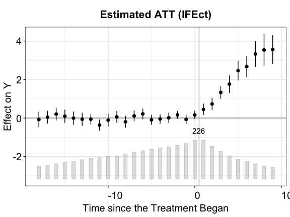
The matrix completion (MC) estimator
For the MC method, we also need to specify a sequence of candidate
tuning parameters. For example, we can specify
lambda = c(1, 0.8, 0.6, 0.4, 0.2, 0.05). If users don’t
have any prior knowledge to set candidate tuning parameters, a number of
candidate tuning parameters can be generated automatically based on the
information from the outcome variable. We specify the number in option
nlambda, e.g. nlambda = 10.
out.mc <- fect(Y ~ D + X1 + X2, data = simdata, index = c("id","time"),
          force = "two-way", method = "mc", CV = TRUE,
          se = TRUE, nboots = 200, parallel = TRUE)
#> Parallel computing ...
#> Cross-validating ...
#> Criterion: Mean Squared Prediction Error
#> Matrix completion method...
#>
#>  lambda.norm = 1.00000; MSPE = 7.02065; MSPTATT = 0.28561; MSE = 5.80999
#>
#>  lambda.norm = 0.42170; MSPE = 5.45943; MSPTATT = 0.12218; MSE = 4.15356
#>
#>  lambda.norm = 0.17783; MSPE = 5.17432; MSPTATT = 0.04007; MSE = 1.57548
#> *
#>
#>  lambda.norm = 0.07499; MSPE = 5.37711; MSPTATT = 0.00815; MSE = 0.28590
#>
#>  lambda.norm = 0.03162; MSPE = 5.63317; MSPTATT = 0.00170; MSE = 0.05133
#>
#>  lambda.norm = 0.01334; MSPE = 6.55505; MSPTATT = 0.00034; MSE = 0.00914
#>
#>
#>  lambda.norm* = 0.177827941003892
#>
#> Bootstrapping for uncertainties ...
#> 200 runs
plot(out.mc, main = "Estimated ATT (MC)")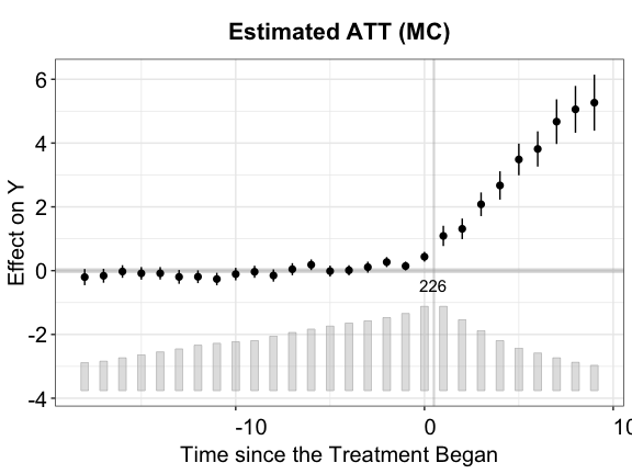
Balanced sample
out.bal <- fect(Y ~ D + X1 + X2, data = simdata, index = c("id","time"),
  balance.period = c(-4, 4), force = "two-way", method = "ife",
  CV = FALSE, r = 2, se = TRUE, nboots = 200, parallel = TRUE)
#> Parallel computing ...
#> Bootstrapping for uncertainties ...
#> 200 runs
plot(out.bal, main = "Estimated ATT (Balanced Sample)")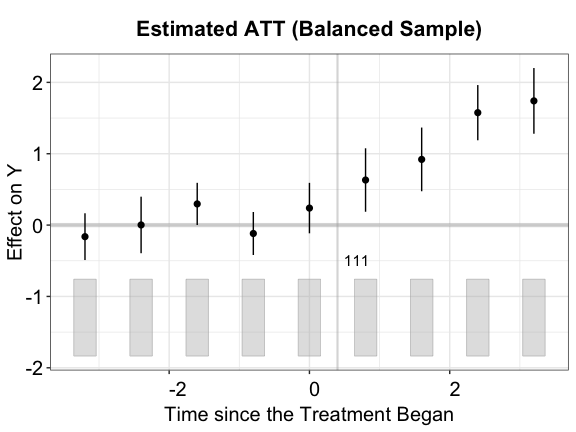
Heterogeneous treatment effects
We provide several methods for researchers to explore heterogeneous treatment effects (HTE)。
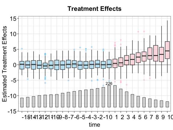
Box plots
One way to understand HTE is to use a series of box plots to
visualize the estimated individualistic treatment effects of
observations under the treatment condition (by setting
type = "box"). Although these effects are not identified at
the individual observation level, their level of dispersion is
informative of treatment effects heterogeneity at different (relative)
time periods, as well as model performance.
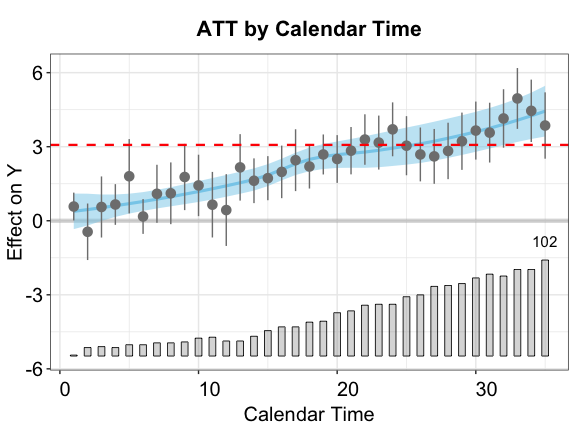
By calendar time
Another way to explore HTE is to investigate how the treatment effect evolves over time. In the plot below, the point estimates represents the ATTs by calendar time; the blue curve and band represent a lowess fit of the estimates and its 95% confidence interval, respectively; and the red horizontal dashed line represents the ATT (averaged over all time periods).
Diagostic tests
We provide three types of diagnostic tests: (1) a placebo test, (2) a test for (no) pretrend, and (3) a test for (no) carry-over effects. For each test, we support both the difference-in-means (DIM) approach and the equivalence approach. The details are provided in the paper.
Placebo tests
We provide a placebo test for a settled model—hence, cross-validation
is not allowed—by setting placeboTest = TRUE. We specify a
range of pretreatment periods as “placebo periods” in option
placebo.period to remove observations in the specified
range for model fitting, and then test whether the estimated ATT in this
range is significantly different from zero. Below, we set
c(-2, 0) as the placebo periods.
out.fect.p <- fect(Y ~ D + X1 + X2, data = simdata, index = c("id", "time"),
  force = "two-way", parallel = TRUE, se = TRUE, CV = 0,
  nboots = 200, placeboTest = TRUE, placebo.period = c(-2, 0))

out.ife.p <- fect(Y ~ D + X1 + X2, data = simdata, index = c("id", "time"),
  force = "two-way", method = "ife",  r = 2, CV = 0,
  parallel = TRUE, se = TRUE,
  nboots = 200, placeboTest = TRUE, placebo.period = c(-2, 0))

out.mc.p <- fect(Y ~ D + X1 + X2, data = simdata, index = c("id", "time"),
  force = "two-way", method = "mc",  lambda = out.mc$lambda.cv,
  CV = 0, parallel = TRUE, se = TRUE,
  nboots = 200, placeboTest = TRUE, placebo.period = c(-2, 0))
The placebo test conducts two types of tests:
t test. If t-test p-value is smaller than a pre-specified threshold (e.g. 5%), we reject the null of no-differences. Hence, the placebo test is deemed failed.
TOST. The TOST checks whether the 90% confidence intervals for estimated ATTs in the placebo period exceed a pre-specified range (defined by a threshold), or the equivalence range. A TOST p-value smaller than a pre-specified threshold suggests that the null of difference bigger than the threshold is rejected; hence, the placebo test is passed.
By default, the plot will display the p-value of the \(t\)-test
(stats = "placebo.p"). Users can also add the p-value of a
corresponding TOST test by setting
stats = c("placebo.p","equiv.p"). A larger placebo p-value
from a t-test and a smaller placebo TOST p-value are preferred.
Users can turn off the dotted plot in placebo periods by setting
vis = "none".
plot(out.ife.p, ylab = "Effect of D on Y", main = "Estimated ATT (IFE)",
     cex.text = 0.8, stats = c("placebo.p","equiv.p"))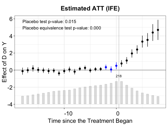
plot(out.mc.p, vis = "none", cex.text = 0.8, stats = c("placebo.p","equiv.p"),
     main = "Estimated ATT (MC)")
The results in the placebo test confirm that IFEct is a better model than MC for this particular DGP.
Tests for (no) pre-trend
We introduce two statistical tests for the presence of a pre-trend (or the lack thereof). The first test is an \(F\) test for zero residual averages in the pretreatment periods. The second test is a two-one-sided \(t\) (TOST) test, a type of equivalence tests.
F test. We offer a goodness-of-fit test (a variant
of the \(F\) test) and to gauge the
presence of pretreatment (differential) trends. A larger F-test p-value
suggests a better pre-trend fitting. Users can specify a test range in
option pre.periods. For example,
pre.periods = c(-4,0) means that we test pretreatment trend
of the last 5 periods prior to the treatment (from period -4 to period
0). If pre.period = NULL (default), all pretreatment
periods in which the number of treated units exceeds the total number of
treated units * proportion will be included in the
test.
TOST. The TOST checks whether the 90% confidence
intervals for estimated ATTs in the pretreatment periods (again, subject
to the proportion option) exceed a pre-specified range, or
the equivalence range. A smaller TOST p-value suggests a better
pre-trend fitting. While users can check the values of confidence
intervals, we give a visualization of the equivalence test. We can plot
the pretreatment residual average with the equivalence confidence
intervals by setting type = "equiv". Option
tost.threshold sets the equivalence range (the default is
\(0.36\sigma_{\epsilon}\) in which
\(\sigma_{\epsilon}\) is the standard
deviation of the outcome variable after two-way fixed effects are
partialed out). By setting range = "both", both the minimum
range (in gray) and the equivalence range (in red) are drawn.
On the topleft corner of the graph, we show several statistics of the
user’s choice. User can choose which statistics to show by setting
stats = c("none", "F.stat", "F.p", "F.equiv.p", "equiv.p")
which corresponds to not showing any, the \(F\) statistic, the p-value for the \(F\) test, the p-value for the equivalence
\(F\) test, the (maximum) p-value for
the the TOST tests, respectively. For the gap plot, the default is
stats = "none". For the equivalence plot, the default is
stats = c("equiv.p, F.p"). Users can also change the labels
of statistics using the stats.labs options. Users can
adjust its position using the stats.pos option, for example
stats.pos = c(-30, 4). To turn off the statistics, set
stats = "none".
Below, we visualize the result of the equivalence test for each of the three estimators using our simulated data. These figures show that both the IFE and MC methods pass the equivalence test while the FE method does not.
plot(out.fect, type = "equiv", ylim = c(-4,4),
     cex.legend = 0.6, main = "Testing Pre-Trend (FEct)", cex.text = 0.8)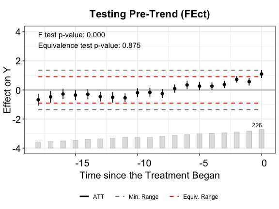
plot(out.ife, type = "equiv", ylim = c(-4,4),
     cex.legend = 0.6, main = "Testing Pre-Trend (IFEct)", cex.text = 0.8)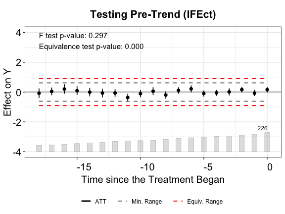
plot(out.mc, type = "equiv", ylim = c(-4,4),
     cex.legend = 0.6, main = "Testing Pre-Trend (MC)", cex.text = 0.8)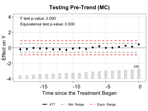
From the above plots, we see that FEct fails both tests; IFEct passes both tests using a conventional test size (5%); and MC fails the F tests, but passes the TOST (equivalence) test. Hence, we may conclude that IFEct is a more suitable model.
Leave-one-out pre-trend test
Instead of using estimated ATTs for periods prior to the treatment to
test for pre-trends, we can use a leave-one-out (LOO) approach
(loo = TRUE) to consecutively hide one pretreatment period
(relative to the timing of the treatment) and repeatedly estimate the
pseudo treatment effects for that pretreatment period. The LOO approach
can be understood as an extension of the placebo test. It has the
benefit of providing users with a more holistic view of whether the
identifying assumptions likely hold. However, as the program needs to
conduct uncertainty estimates for each turn, it is much more
time-consuming than the original one.
out.fect.loo <- fect(Y ~ D + X1 + X2, data = simdata, index = c("id","time"),
  method = "fe", force = "two-way", se = TRUE, parallel = TRUE, nboots = 200, loo = TRUE)
out.ife.loo <- fect(Y ~ D + X1 + X2, data = simdata, index = c("id","time"),
  method = "ife", force = "two-way", se = TRUE, parallel = TRUE, nboots = 200, loo = TRUE)
out.mc.loo <- fect(Y ~ D + X1 + X2, data = simdata, index = c("id","time"),
  method = "mc", force = "two-way", se = TRUE, parallel = TRUE, nboots = 200, loo = TRUE)
After the LOO estimation, one can plot these LOO pre-trends in the
gap plot or the equivalence plot by setting loo = TRUE in
the plot function.
plot(out.fect.loo, type = "equiv", ylim = c(-4,4), loo = TRUE,
     cex.legend = 0.6, main = "Testing Pre-Trend LOO (FEct)", cex.text = 0.8)

plot(out.ife.loo, type = "equiv", ylim = c(-4,4), loo = TRUE,
     cex.legend = 0.6, main = "Testing Pre-Trend LOO (IFEct)", cex.text = 0.8)

plot(out.mc.loo, type = "equiv", ylim = c(-4,4), loo = TRUE,
     cex.legend = 0.6, main = "Testing Pre-Trend LOO (MC)", cex.text = 0.8)
Note that the LOO test usually takes lots of computational power. For our example, we find that the IFE estimator still passes both the F test and the equivalence test based on its LOO pre-trends, while the MC estimator fails both tests.
Exiting the treatment
fect allows the treatment to switch back and forth
and provides diagnostic tools for this setting. After the estimation, we
can visualize the period-wise ATTs relative to the exit
of treatments by setting type = "exit" (one can still draw
the classic gap plot by setting type = "gap"). The x-axis
is then realigned based on the timing of the treatment’s exit, not
onset, e.g., 1 represents 1 period after the treatment ends.
plot(out.fect, type = "exit", ylim = c(-2.5,4.5), main = "What Happens after the Treatment Switches Off?")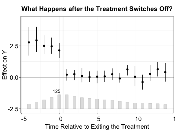
Tests for (no) carryover effects
The idea of the placebo test can be extended to testing the presence
of carryover effects. Instead of hiding a few periods right before the
treatment starts, we hide a few periods right after the treatment ends.
If carryover effects do not exist, we would expect the average
prediction error in those periods to be close to zero. To perform the
carryover test, we set the option carryoverTest = TRUE. We
can treat a range of exit-treatment periods in option
carryover.period to remove observations in the specified
range for model fitting, and then test whether the estimated ATT in this
range is significantly different from zero.
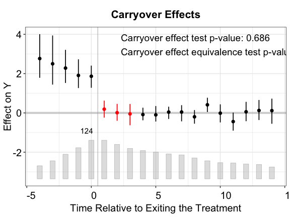
Below, we set carryover.period = c(1, 3). As we deduct
the treatment effect from the outcome in simdata, we
expect the average prediction error for these removed periods to be
close to zero.
out.fect.c <- fect(Y ~ D + X1 + X2, data = simdata, index = c("id", "time"),
  force = "two-way", parallel = TRUE, se = TRUE, CV = 0,
  nboots = 200, carryoverTest = TRUE, carryover.period = c(1, 3))

out.ife.c <- fect(Y ~ D + X1 + X2, data = simdata, index = c("id", "time"),
  force = "two-way", method = "ife", r = 2, CV = 0,
  parallel = TRUE, se = TRUE,
  nboots = 200, carryoverTest = TRUE, carryover.period = c(1, 3))

out.mc.c <- fect(Y ~ D + X1 + X2, data = simdata, index = c("id", "time"),
  force = "two-way", method = "mc",  lambda = out.mc$lambda.cv,
  CV = 0, parallel = TRUE, se = TRUE,
  nboots = 200, carryoverTest = TRUE, carryover.period = c(1, 3))
Like the placebo test, the plot will display the p-value of the
carryover effect test (stats = "carryover.p"). Users can
also add the p-value of a corresponding TOST test by setting
stats = c("carryover.p","equiv.p").
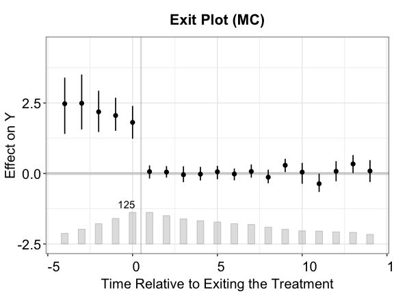
plot(out.fect.c, type = "exit", ylim = c(-2.5,4.5),
          cex.text = 0.8, main = "Carryover Effects (FE)")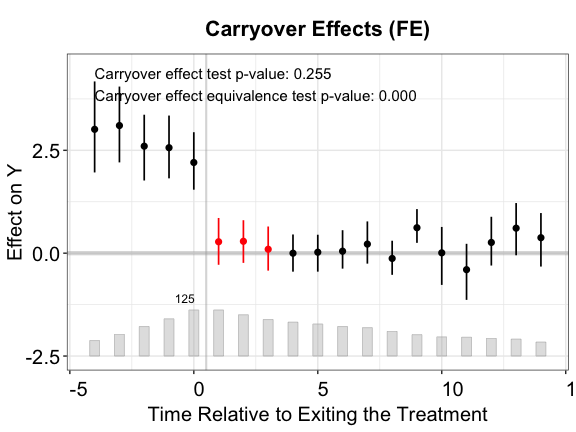
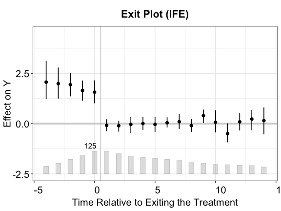
plot(out.ife.c, type = "exit", ylim = c(-2.5,4.5),
          cex.text = 0.8, main = "Carryover Effects (IFE)")
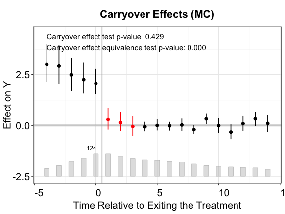
Once again, the IFE estimator outperforms the other two.
Using real-world data, researchers will likely find that carryover
effects exist. If such effects are limited, researchers can consider
removing a few periods after the treatment ended for the treated units
from the first-stage estimation (using the carryover.period
option) and re-estimated the model (and re-conduct the test). We provide
such an example in the paper. Here, we illustrate the option using
simdata.
out.ife.rm.test <- fect(Y ~ D + X1 + X2, data = simdata, index = c("id", "time"),
  force = "two-way", method = "ife", r = 2, CV = 0,
  parallel = TRUE, se = TRUE,  carryover.rm = 3,
  nboots = 200, carryoverTest = TRUE, carryover.period = c(1, 3))# remove three periods

plot(out.ife.rm.test, cex.text = 0.8, stats.pos = c(7, 2.5))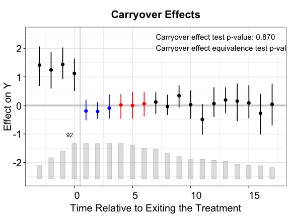
In the above plot, the three periods in blue are droppred from the first-stage estimation of the factor model while the periods in red are reserved for the (no) carryover effects test.
Other options
We provide a few other options for estimation and visualization.
More visualization options
The plot() function shipped in fect offers some options that help to improve the visualization.
We can remove the bar plot at the bottom of the plot by setting
count = FALSE
plot(out.ife, count = FALSE)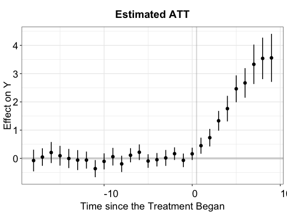
By setting the option show.points = TRUE, we visualize
the estimated period-wise ATTs as well as their uncertainty estimates in
point-wise vertical intervals. The shorter interval at each point
corresponds to the 90% confidence interval of ATT while the longer
interval corresponds to the 95% confidence interval.
plot(out.ife, show.points = TRUE)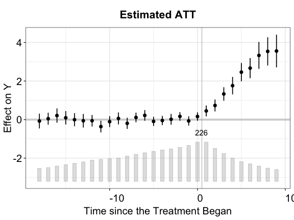
plot(out.ife.p, show.points = TRUE)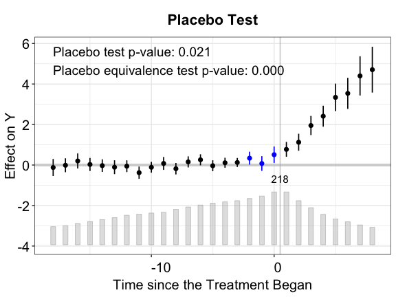
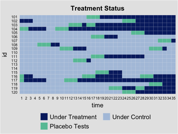
By setting the option type = "status", we can visualize
the treatment status of all observations. We only present the label of
the time by setting axis.lab = "time".
plot(out.fect, type = 'status', axis.lab = "time", cex.axis = 0.6)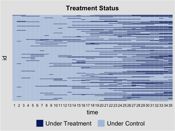
For the placebo test, the manually hided observations are marked in
cyan. We can show only a sub-group’s treatment status by specifying the
option id to certain units.
For the carryover test, the manually hidden observations are marked
in light red. We can also move grid lines by setting
gridOff = TRUE.
plot(out.fect.c, type = 'status', axis.lab = "off", gridOff = TRUE)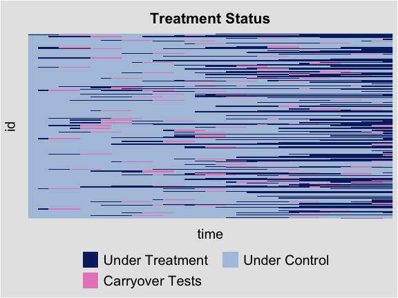
For the carryover test with removed observation, the removed observations are marked in yellow.
plot(out.ife.rm.test, type = 'status', axis.lab = "off", gridOff = TRUE)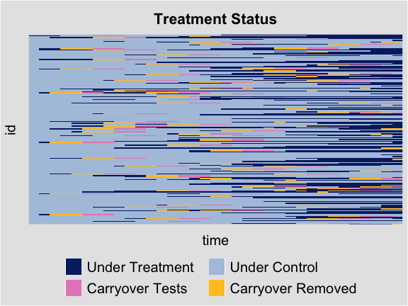
Average cohort effect
fect allows us to estimate and visualize the ATTs for sub-groups of treated units. For example, it can draw the gap plot for units that adopt the treatment at the same time under staggered adoption, which is defined as “Cohort” in Sun and Abraham (2021). Our simulated dataset is not ideal to demonstrate this functionality because the treatment switches on and off. To improve feasibility, we define a cohort as a group of treated units that first adopt the treatment at the same time.
panelview(Y ~ D, data = simdata, index = c("id","time"), by.timing = TRUE,
  axis.lab = "time", xlab = "Time", ylab = "Unit",
  background = "white", main = "Simulated Data: Treatment Status")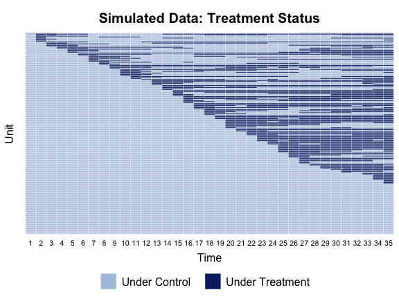
The function get.cohort() shipped in fect can generate a new variable “Cohort” based on the timing when treated units first get treated.
simdata.cohort <- get.cohort(data = simdata,D = 'D',index = c("id","time"))
print(table(simdata.cohort[,'Cohort']))
#>
#>  Cohort:1 Cohort:10 Cohort:11 Cohort:12 Cohort:13 Cohort:14 Cohort:15 Cohort:16
#>        35       245       105        35       175       175       210       245
#> Cohort:17 Cohort:18 Cohort:19  Cohort:2 Cohort:20 Cohort:21 Cohort:22 Cohort:23
#>       210       210       140       280       315       105       140       210
#> Cohort:24 Cohort:25 Cohort:26 Cohort:27 Cohort:28 Cohort:29  Cohort:3 Cohort:30
#>       105       280       175       210        70       105       175        35
#> Cohort:31 Cohort:33 Cohort:34 Cohort:35  Cohort:4  Cohort:5  Cohort:6  Cohort:7
#>       105        70       175       140        70       140       105       210
#>  Cohort:8  Cohort:9   Control
#>       105       140      1750
We can also pass a list of intervals for first
get-treated time into the entry.time option of
get.cohort(). For example, we can categorize all
treated units into the group that adopts the treatment between time 21
and 27, and the group that adopts the treatment in time 30 and 33.
simdata.cohort2 <- get.cohort(data = simdata,D = 'D',index = c("id","time"),
                               entry.time = list(c(21,27),c(30,33)))
print(table(simdata.cohort2[,'Cohort']))
#>
#> Cohort:21-27 Cohort:30-33 Cohort:Other      Control
#>         1225          210         3815         1750
By setting the option group = "Cohort",
fect estimates the ATT for each specified sub-group and
saves it for further visualization.
out.ife.g <- fect(Y ~ D + X1 + X2, data = simdata.cohort, index = c("id","time"),
          force = "two-way", method = "ife", CV = TRUE, r = c(0, 5),
          se = TRUE, nboots = 200, parallel = TRUE, group = 'Cohort')
out.ife.g.p <- fect(Y ~ D + X1 + X2, data = simdata.cohort, index = c("id","time"),
          force = "two-way", method = "ife", CV = FALSE,
          placeboTest = TRUE, placebo.period = c(-2,0),
          se = TRUE, nboots = 200, parallel = TRUE, group = 'Cohort')
Then one can draw the gap plot, as well as the equivalence plot, for each sub-group. Here we present the gap plot for Cohort 22.
Other estimators
The logic of imputation estimator can be extended to more settings.
Complex Fixed Effects. When there exists more
dimensions of fixed effects in addition to the unit and time fixed
effects, we can resort to the “cfe”(complex fixed
effects) estimator to impute the counterfactual based on a linear model
with multiple levels of fixed effects. It accepts two options:
sfe specifies simple (additive) fixed effects in addition
to the unit and time fixed effects and cfe receives a
list object and each component in the list is a vector of
length 2. The value of the first element of each component is the name
of group variable for which fixed effects are to be estimated
(e.g. unit names); the value of the second element is the name of a
regressor (e.g., a time trend). For example, we can estimate a model
with an additional fixed effects FE3 along with a
unit-specific time trend.
simdata[,"FE3"] <- sample(c(1,2,3,4,5), size = dim(simdata)[1], replace = TRUE)
out.cfe <- fect(Y ~ D + X1 + X2, data = simdata, index = c("id","time"),
  method = "cfe", force = "two-way", se = TRUE, parallel = TRUE, nboots = 200,
  sfe = c("FE3"), cfe = list(c("id","time")))
plot(out.cfe)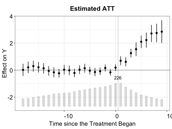
Polynomial. When only need to include unit-specific
time trends, we can use the “polynomial” estimator. By
setting degree = 2, we can estimate the ATT based on a
linear model with unit and time fixed effects, along with a
unit-specific time trend and quadratic time trend.
out.poly <- fect(Y ~ D + X1 + X2, data = simdata, index = c("id","time"),
  method = "polynomial", force = "two-way", se = TRUE, parallel = TRUE, nboots = 200,
  degree = 2)
plot(out.poly)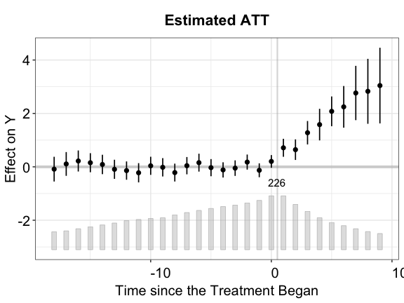
Additional Notes
By default, the program will drop the units that have no larger than 5 observations under control, which is the reason why sometimes there are less available units in the placebo test or carryover test than in the original estimation. We can specify a preferred criteria in the option
min.T0(default to 5). As a rule of thumb for the IFE estimator, the minimum number of observations under control for a unit should be larger than the specified number of factorr.We can get replicable results by setting the option
seedto a certain integer, no matter whether the parallel computing is used.When
na.rm = FALSE(default), the program allows observations to have missing outcomes \(Y\) or covariates \(X\) but decided treatment statuses \(D\). Otherwise the program will drop all observations that have missing values in outcomes, treatments, or covariates.