3 Continuous G
This chapter demonstrates FDID estimation when the baseline factor \(G\) is continuous, using lnpczupu (log genealogy book density) as the treatment variable.
Note: Continuous \(G\) currently supports only the linear estimators ("did", "ols1", "ols2"). Methods that require binary group membership — "ebal", "ipw", "aipw" — are not available. Support will be extended in future versions.
3.1 Setup
mortality$uniqueid <- paste(as.character(mortality$provid),
                            as.character(mortality$countyid), sep = "-")

covar      <- c("avggrain", "nograin", "urban", "dis_bj", "dis_pc",
                "rice", "minority", "edu", "lnpop")
tr_period  <- 1958:1961
ref_period <- 1957
Prepare the data using lnpczupu as the continuous \(G\):
s_cont <- fdid_prepare(
  data       = transform(mortality, G = lnpczupu),
  Y_label    = "mortality",
  X_labels   = covar,
  G_label    = "G",
  unit_label = "uniqueid",
  time_label = "year"
)
3.2 Estimation
3.2.1 DID (no covariates)
result_cont_did <- fdid(s_cont, tr_period = tr_period, ref_period = ref_period,
                        method = "did")
summary(result_cont_did)
#>
#>   Factorial Difference-in-Differences (FDID) Summary
#>   ════════════════════════════════════════════════════════════════════════
#>   Method:             did
#>   Variance Type:      robust
#>   Reference Period:   1957
#>   Pre-Event Period:   1954, 1955, 1956, 1957
#>   Event Period:       1958, 1959, 1960, 1961
#>   Post-Event Period:  1962, 1963, 1964, 1965, 1966
#>   ════════════════════════════════════════════════════════════════════════
#>
#>   Aggregate Estimates
#>   ────────────────────────────────────────────────────────────────────────
#>                       Estimate    Std.Error     95% CI
#>   ────────────────────────────────────────────────────────────────────────
#>   Pre-Event             1.0217       0.4968  [0.0466, 1.9968]
#>   Event                -5.8461       0.9664  [-7.7427, -3.9494]
#>   Post-Event           -1.8229       0.4206  [-2.6483, -0.9975]
#>   ────────────────────────────────────────────────────────────────────────
#>
#>   Dynamic Estimates
#>   ────────────────────────────────────────────────────────────────────────
#>                       Estimate    Std.Error     95% CI
#>   ────────────────────────────────────────────────────────────────────────
#>   1954                  2.1510       0.6306  [0.9135, 3.3886]
#>   1955                  1.0158       0.7323  [-0.4213, 2.4529]
#>   1956                 -0.1018       0.4045  [-0.8956, 0.6921]
#>   1957                  0.0000       0.0000  [0.0000, 0.0000]
#>    ····································································
#>   1958                 -2.2174       0.8346  [-3.8553, -0.5795]
#>   1959                 -6.6445       1.2558  [-9.1091, -4.1799]
#>   1960                -11.4351       1.9000  [-15.1640, -7.7062]
#>   1961                 -3.0872       0.9743  [-4.9993, -1.1751]
#>    ····································································
#>   1962                 -0.3202       0.5569  [-1.4131, 0.7727]
#>   1963                 -2.4654       0.4192  [-3.2880, -1.6427]
#>   1964                 -2.8375       0.4930  [-3.8051, -1.8698]
#>   1965                 -1.7812       0.4492  [-2.6628, -0.8997]
#>   1966                 -1.7103       0.4592  [-2.6115, -0.8092]
#>   ────────────────────────────────────────────────────────────────────────
3.2.2 OLS without interactions
result_cont_ols1 <- fdid(s_cont, tr_period = tr_period, ref_period = ref_period,
                         method = "ols1")
summary(result_cont_ols1)
#>
#>   Factorial Difference-in-Differences (FDID) Summary
#>   ════════════════════════════════════════════════════════════════════════
#>   Method:             ols1
#>   Variance Type:      robust
#>   Reference Period:   1957
#>   Pre-Event Period:   1954, 1955, 1956, 1957
#>   Event Period:       1958, 1959, 1960, 1961
#>   Post-Event Period:  1962, 1963, 1964, 1965, 1966
#>   ════════════════════════════════════════════════════════════════════════
#>
#>   Aggregate Estimates
#>   ────────────────────────────────────────────────────────────────────────
#>                       Estimate    Std.Error     95% CI
#>   ────────────────────────────────────────────────────────────────────────
#>   Pre-Event             0.6893       0.5214  [-0.3341, 1.7126]
#>   Event               -10.1637       1.4352  [-12.9804, -7.3470]
#>   Post-Event           -1.8209       0.4384  [-2.6813, -0.9606]
#>   ────────────────────────────────────────────────────────────────────────
#>
#>   Dynamic Estimates
#>   ────────────────────────────────────────────────────────────────────────
#>                       Estimate    Std.Error     95% CI
#>   ────────────────────────────────────────────────────────────────────────
#>   1954                  1.2664       0.7097  [-0.1265, 2.6593]
#>   1955                  0.7986       0.7296  [-0.6333, 2.2305]
#>   1956                  0.0028       0.4575  [-0.8950, 0.9006]
#>   1957                  0.0000       0.0000  [0.0000, 0.0000]
#>    ····································································
#>   1958                 -4.2568       0.9149  [-6.0523, -2.4613]
#>   1959                -12.5895       2.0838  [-16.6792, -8.4998]
#>   1960                -19.5046       2.7515  [-24.9046, -14.1045]
#>   1961                 -4.3040       1.2534  [-6.7638, -1.8441]
#>    ····································································
#>   1962                 -1.1326       0.7267  [-2.5588, 0.2936]
#>   1963                 -2.0553       0.4422  [-2.9231, -1.1874]
#>   1964                 -2.6525       0.5118  [-3.6570, -1.6480]
#>   1965                 -1.6514       0.4613  [-2.5567, -0.7462]
#>   1966                 -1.6129       0.4824  [-2.5597, -0.6662]
#>   ────────────────────────────────────────────────────────────────────────
3.2.3 OLS with interactions (OLS\(_*\))
result_cont_ols2 <- fdid(s_cont, tr_period = tr_period, ref_period = ref_period,
method = "ols2")
summary(result_cont_ols2)
#>
#> Factorial Difference-in-Differences (FDID) Summary
#> ════════════════════════════════════════════════════════════════════════
#> Method: ols2
#> Variance Type: robust
#> Reference Period: 1957
#> Pre-Event Period: 1954, 1955, 1956, 1957
#> Event Period: 1958, 1959, 1960, 1961
#> Post-Event Period: 1962, 1963, 1964, 1965, 1966
#> ════════════════════════════════════════════════════════════════════════
#>
#> Aggregate Estimates
#> ────────────────────────────────────────────────────────────────────────
#> Estimate Std.Error 95% CI
#> ────────────────────────────────────────────────────────────────────────
#> Pre-Event -0.5072 0.9389 [-2.3474, 1.3329]
#> Event -5.1507 2.6137 [-10.2737, -0.0278]
#> Post-Event -1.3462 0.5597 [-2.4432, -0.2492]
#> ────────────────────────────────────────────────────────────────────────
#>
#> Dynamic Estimates
#> ────────────────────────────────────────────────────────────────────────
#> Estimate Std.Error 95% CI
#> ────────────────────────────────────────────────────────────────────────
#> 1954 0.0006 1.0572 [-2.0715, 2.0728]
#> 1955 -0.6477 1.1064 [-2.8162, 1.5208]
#> 1956 -0.8746 1.0022 [-2.8389, 1.0896]
#> 1957 0.0000 0.0000 [0.0000, 0.0000]
#> ····································································
#> 1958 -3.2263 1.1839 [-5.5468, -0.9057]
#> 1959 -5.5528 3.9086 [-13.2136, 2.1080]
#> 1960 -10.9466 4.1922 [-19.1634, -2.7298]
#> 1961 -0.8773 3.2515 [-7.2501, 5.4956]
#> ····································································
#> 1962 1.1766 1.4156 [-1.5979, 3.9511]
#> 1963 -2.2845 0.9383 [-4.1237, -0.4454]
#> 1964 -2.0729 0.8323 [-3.7043, -0.4415]
#> 1965 -1.7336 0.6987 [-3.1031, -0.3640]
#> 1966 -1.8167 1.0155 [-3.8071, 0.1738]
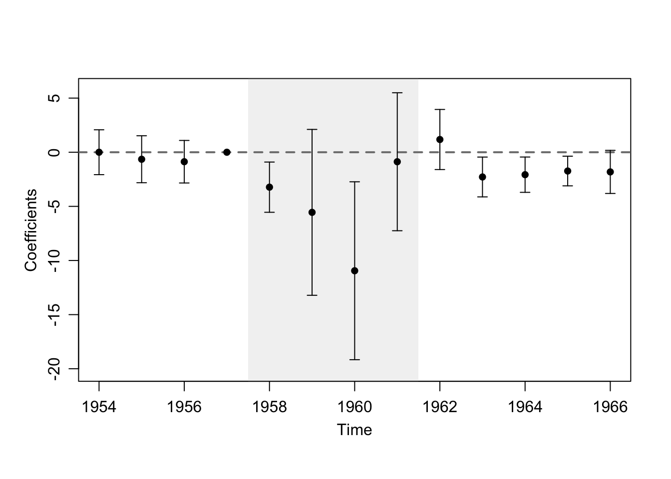
#> ────────────────────────────────────────────────────────────────────────3.3 Plots
plot(result_cont_ols2, type = "raw")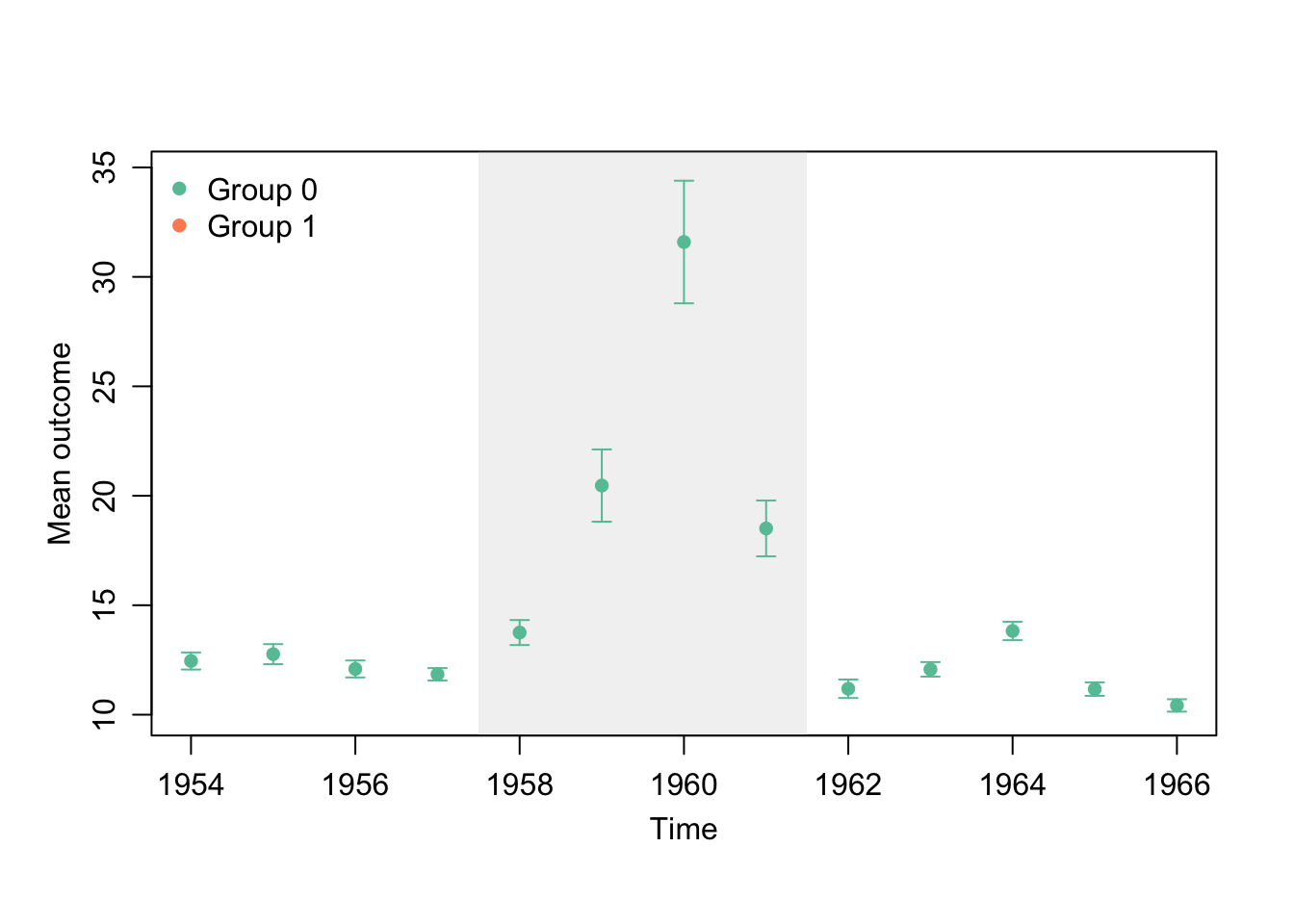
plot(result_cont_ols2, type = "dynamic")