2 Binary G
In this chapter, we outline the complete workflow for an FDID analysis, which includes preparing the dataset, performing the estimation, and plotting the results.
2.1 Data preparation
Before calling fdid_prepare(), make sure
- each unit has a unique identifier across time;
- the baseline factor \(G\) is coded as a 0/1 variable. To match the current implementation (binary \(G\)), we define
- \(G=1\) for counties above the median social-capital measure;
- \(G=0\) for counties below the median.
mortality$uniqueid <- paste(as.character(mortality$provid), as.character(mortality$countyid), sep = "-")
mortality$G <- ifelse(mortality$pczupu >= median(mortality$pczupu, na.rm = TRUE), 1, 0)
Next, define the key input parameters (event window, reference period, variable names):
tr_period <- 1958:1961
ref_period <- 1957
treat <- "G"
Y <- "mortality"
time <- "year"
unit <- "uniqueid"
covar <- c("avggrain", "nograin", "urban", "dis_bj", "dis_pc",
           "rice", "minority", "edu", "lnpop")
Finally, the user can use fdid_prepare() to reshape long-format panel data into a wide-format dataset and to construct the ingredients needed by fdid(). It also averages time-varying covariates and standardizes naming so downstream steps are consistent.
prepared_d <- fdid_prepare(
  data = mortality,
  Y_label = Y,
  X_labels = covar,
  G_label = treat,
  unit_label = unit,
  time_label = time
)head(prepared_d)Currently, the package accepts only long-format data; if the data are already in wide format, the user must convert them to long format first.
2.1.1 Clustering if needed
Since the estimation program operates on the wide format and each row represents one unit, the robust standard errors we’re using are analogous to clustering at the unit level. However, if needed, the user can choose a different and higher level to cluster by passing the cluster variable (e.g. provid) to fdid_prepare(). Then fdid(..., vartype="robust") will report robust standard errors clustered at the higher level.
prepared_d_cl_prov <- fdid_prepare(
  data = mortality,
  Y_label = Y,
  X_labels = covar,
  G_label = treat,
  unit_label = unit,
  time_label = time,
  cluster_label = "provid"
)
2.2 FDID: A quick review
fdid() performs factorial difference-in-differences (FDID) estimation using cross-sectional estimation methods based on first differences. It converts the \((Y_{i,t}, G_i, X_i)\) into a cross-sectional form \((\Delta Y_i, G_i, X_i)\) by comparing each period (or average of a time window) to a reference period.
fdid() reports both aggregate and dynamic estimates with different definition of \(Y_{i,*}\) in \(\Delta Y_i=Y_{i,*}-Y_{i,\text{ref}}\):
- Aggregate estimates:
- Pre-event average effect for all pre-event periods excluding the reference period: \(Y_{i,*}=\bar Y_{i,\text{pre}}\) where \(\bar Y_{i,\text{pre}}\) is the average of \(Y_{i,t}\) across all pre-event periods except the reference period.
- Event-period average effect for all event periods: \(Y_{i,*}=\bar Y_{i,\text{event}}\) where \(\bar Y_{i,\text{event}}\) is the average of \(Y_{i,t}\) across all event periods.
- Post-event average effect for all post-event periods: \(Y_{i,*}=\bar Y_{i,\text{post}}\) where \(\bar Y_{i,\text{post}}\) is the average of \(Y_{i,t}\) across all post-event periods.
- Dynamic Estimates:
- Dynamic period-by-period estimates relative to the reference: \(Y_{i,*}=Y_{i,t}\) for all \(t\).
How periods are defined: tr_period defines the event window. Every period before it is “pre”, every period after it is “post”. The reference period is separately set by ref_period and does not have to be the last pre-event period. If it’s set in event or post-event window, the corresponding window average effect will also exclude the reference period when calculating the average.
Carryout effect: Because we cannot rule out carryover effects, all periods during or after the event should be considered treated or exposed. Therefore, setting a post-event period as the reference period is not recommended, even though we report separate estimates for the event and post-event periods.
Compared with the TWFE model, our approach
- forces each period-by-period estimation to use a balanced two-period comparison;
- makes it easy to plug in selection-on-observables tools (stratification, balancing, matching, IPW, AIPW, outcome modeling, double machine learning, etc.).
The reason why OLS is problematic here is the same as the issue with running a two-way fixed effects (TWFE) model using long-format data such as the violation of the no anticipation assumption.
2.3 Estimation
Use method to choose an estimator:
-
"did": OLS without covariates (i.e. \(2\times2\) DID). -
"ols1": OLS with covariates but no interactions, equivalent to conventional two-way fixed effects (TWFE) -
"ols2": OLS with covariates and interactions, equivalent to TWFE with three-way interactions -
"ebal": Entropy balancing. -
"ipw": IPW via generalized random forests. -
"aipw": AIPW via generalized random forests.
Default is ols1.
2.3.1 Difference-in-Differences
By setting method = 'did', the estimated model is the no-covariate specification: \[
\Delta Y_i=\beta_0+\beta_G G_i+\varepsilon_i
\] Here, \(\beta_G\) is a cross-sectional analogue of the canonical \(2\times2\) DID estimand.
fdid_results_did <- fdid(
  s = prepared_d,
  tr_period = tr_period,
  ref_period = ref_period,
  method = "did",
  vartype = "robust",
)
summary() reports the point estimates, standard errors and 95% confidence intervals for aggregate estimates and dynamic estimates:
summary(fdid_results_did)
#>
#>   Factorial Difference-in-Differences (FDID) Summary
#>   ════════════════════════════════════════════════════════════════════════
#>   Method:             did
#>   Variance Type:      robust
#>   Reference Period:   1957
#>   Pre-Event Period:   1954, 1955, 1956, 1957
#>   Event Period:       1958, 1959, 1960, 1961
#>   Post-Event Period:  1962, 1963, 1964, 1965, 1966
#>   ════════════════════════════════════════════════════════════════════════
#>
#>   Aggregate Estimates
#>   ────────────────────────────────────────────────────────────────────────
#>                       Estimate    Std.Error     95% CI
#>   ────────────────────────────────────────────────────────────────────────
#>   Pre-Event             0.3220       0.2161  [-0.1022, 0.7461]
#>   Event                -2.3163       0.7902  [-3.8671, -0.7654]
#>   Post-Event           -0.8068       0.2039  [-1.2071, -0.4066]
#>   ────────────────────────────────────────────────────────────────────────
#>
#>   Dynamic Estimates
#>   ────────────────────────────────────────────────────────────────────────
#>                       Estimate    Std.Error     95% CI
#>   ────────────────────────────────────────────────────────────────────────
#>   1954                  1.0497       0.3191  [0.4234, 1.6760]
#>   1955                  0.0489       0.2765  [-0.4936, 0.5915]
#>   1956                 -0.1327       0.2391  [-0.6020, 0.3366]
#>   1957                  0.0000       0.0000  [0.0000, 0.0000]
#>    ····································································
#>   1958                 -0.3542       0.3919  [-1.1234, 0.4149]
#>   1959                 -2.3814       1.0539  [-4.4497, -0.3131]
#>   1960                 -4.9775       1.7324  [-8.3774, -1.5776]
#>   1961                 -1.5519       0.7255  [-2.9759, -0.1280]
#>    ····································································
#>   1962                 -0.1102       0.2736  [-0.6471, 0.4268]
#>   1963                 -0.9441       0.2596  [-1.4536, -0.4346]
#>   1964                 -1.4063       0.2613  [-1.9192, -0.8934]
#>   1965                 -0.8850       0.2204  [-1.3175, -0.4524]
#>   1966                 -0.6887       0.2221  [-1.1246, -0.2529]
#>   ────────────────────────────────────────────────────────────────────────
2.3.2 OLS without interactions
By setting method = "ols1", the estimated model corresponds to the \(OLS_+\) specification in Xu et al. (2026): \[
\Delta Y_i=\beta_0+\beta_GG_i+\beta_X'\mathbf{X}_i+\varepsilon_i
\]
fdid_results_ols1 <- fdid(
  s = prepared_d,
  tr_period = tr_period,
  ref_period = ref_period,
  vartype = "robust",
)summary(fdid_results_ols1)
#>
#> Factorial Difference-in-Differences (FDID) Summary
#> ════════════════════════════════════════════════════════════════════════
#> Method: ols1
#> Variance Type: robust
#> Reference Period: 1957
#> Pre-Event Period: 1954, 1955, 1956, 1957
#> Event Period: 1958, 1959, 1960, 1961
#> Post-Event Period: 1962, 1963, 1964, 1965, 1966
#> ════════════════════════════════════════════════════════════════════════
#>
#> Aggregate Estimates
#> ────────────────────────────────────────────────────────────────────────
#> Estimate Std.Error 95% CI
#> ────────────────────────────────────────────────────────────────────────
#> Pre-Event 0.3334 0.2103 [-0.0793, 0.7462]
#> Event -2.8024 0.7511 [-4.2766, -1.3283]
#> Post-Event -0.4893 0.2025 [-0.8866, -0.0920]
#> ────────────────────────────────────────────────────────────────────────
#>
#> Dynamic Estimates
#> ────────────────────────────────────────────────────────────────────────
#> Estimate Std.Error 95% CI
#> ────────────────────────────────────────────────────────────────────────
#> 1954 0.9565 0.2716 [0.4235, 1.4896]
#> 1955 0.2512 0.2663 [-0.2715, 0.7740]
#> 1956 -0.2074 0.2697 [-0.7367, 0.3218]
#> 1957 0.0000 0.0000 [0.0000, 0.0000]
#> ····································································
#> 1958 -0.8928 0.3800 [-1.6386, -0.1470]
#> 1959 -3.5169 1.1051 [-5.6857, -1.3481]
#> 1960 -5.6338 1.6781 [-8.9271, -2.3404]
#> 1961 -1.1662 0.7263 [-2.5915, 0.2592]
#> ····································································
#> 1962 -0.1948 0.3285 [-0.8395, 0.4499]
#> 1963 -0.5807 0.2601 [-1.0911, -0.0703]
#> 1964 -0.7401 0.2537 [-1.2380, -0.2421]
#> 1965 -0.4843 0.2185 [-0.9131, -0.0555]
#> 1966 -0.4466 0.2183 [-0.8751, -0.0180]
#> ────────────────────────────────────────────────────────────────────────2.3.3 OLS with interactions
By setting method = "ols2", the estimated model corresponds to the \(OLS_*\) specification: \[
\Delta Y_i=\beta_0+\beta_GG_i+\beta_X'\mathbf{X}_i+\beta'_{GX}G_i\mathbf{X}_i+\varepsilon_i
\]
fdid() automatically centers covariates before estimation. With centered \(X_i\), the coefficient on \(G_i\) can be interpreted as consistent estimator for marginal estimand \(\tau_{\text{DID-X}}\) discussed in Xu et al. (2026). The standard error for ols2 with target.pop = "all" (the default) includes the Lin (2013) super-population correction \(\hat{\gamma}'\hat{\Sigma}_X\hat{\gamma}/n\), where \(\hat{\gamma}\) are the estimated interaction coefficients and \(\hat{\Sigma}_X\) is the sample covariance of the covariates.
fdid_results_ols2 <- fdid(
  s = prepared_d,
  tr_period = tr_period,
  ref_period = ref_period,
  method = "ols2",
  vartype = "robust",
)summary(fdid_results_ols2)
#>
#> Factorial Difference-in-Differences (FDID) Summary
#> ════════════════════════════════════════════════════════════════════════
#> Method: ols2
#> Variance Type: robust
#> Reference Period: 1957
#> Pre-Event Period: 1954, 1955, 1956, 1957
#> Event Period: 1958, 1959, 1960, 1961
#> Post-Event Period: 1962, 1963, 1964, 1965, 1966
#> ════════════════════════════════════════════════════════════════════════
#>
#> Aggregate Estimates
#> ────────────────────────────────────────────────────────────────────────
#> Estimate Std.Error 95% CI
#> ────────────────────────────────────────────────────────────────────────
#> Pre-Event 0.3522 0.2193 [-0.0776, 0.7820]
#> Event -2.9264 0.8010 [-4.4963, -1.3564]
#> Post-Event -0.5085 0.2142 [-0.9283, -0.0888]
#> ────────────────────────────────────────────────────────────────────────
#>
#> Dynamic Estimates
#> ────────────────────────────────────────────────────────────────────────
#> Estimate Std.Error 95% CI
#> ────────────────────────────────────────────────────────────────────────
#> 1954 0.9948 0.2827 [0.4407, 1.5488]
#> 1955 0.2735 0.2831 [-0.2814, 0.8284]
#> 1956 -0.2116 0.2731 [-0.7469, 0.3237]
#> 1957 0.0000 0.0000 [0.0000, 0.0000]
#> ····································································
#> 1958 -0.9479 0.3974 [-1.7268, -0.1690]
#> 1959 -3.5576 1.1710 [-5.8528, -1.2625]
#> 1960 -5.7909 1.7526 [-9.2260, -2.3558]
#> 1961 -1.4090 0.7818 [-2.9413, 0.1233]
#> ····································································
#> 1962 -0.1545 0.3646 [-0.8691, 0.5601]
#> 1963 -0.6250 0.2691 [-1.1523, -0.0976]
#> 1964 -0.8070 0.2717 [-1.3394, -0.2745]
#> 1965 -0.5088 0.2273 [-0.9544, -0.0632]
#> 1966 -0.4475 0.2268 [-0.8920, -0.0029]
#> ────────────────────────────────────────────────────────────────────────2.3.4 Entropy balancing
By setting method = "ebal", the estimation program reweights the \(G=0\) group so that its covariate moments match the \(G=1\) group, and then estimates the effect on \(\Delta Y\). Because the weights are constructed to match the \(G=1\) group, this method currently targets \(G=1\) group, so the user must set target.pop = "1".
fdid_results_ebal <- fdid(
  s = prepared_d,
  tr_period = tr_period,
  ref_period = ref_period,
  method = "ebal",
  vartype = "robust",
  target.pop = "1"
)summary(fdid_results_ebal)
#>
#> Factorial Difference-in-Differences (FDID) Summary
#> ════════════════════════════════════════════════════════════════════════
#> Method: ebal
#> Variance Type: robust
#> Reference Period: 1957
#> Pre-Event Period: 1954, 1955, 1956, 1957
#> Event Period: 1958, 1959, 1960, 1961
#> Post-Event Period: 1962, 1963, 1964, 1965, 1966
#> ════════════════════════════════════════════════════════════════════════
#>
#> Aggregate Estimates
#> ────────────────────────────────────────────────────────────────────────
#> Estimate Std.Error 95% CI
#> ────────────────────────────────────────────────────────────────────────
#> Pre-Event 0.5161 0.2453 [0.0347, 0.9975]
#> Event -3.1232 0.9854 [-5.0572, -1.1893]
#> Post-Event -0.5271 0.2081 [-0.9355, -0.1186]
#> ────────────────────────────────────────────────────────────────────────
#>
#> Dynamic Estimates
#> ────────────────────────────────────────────────────────────────────────
#> Estimate Std.Error 95% CI
#> ────────────────────────────────────────────────────────────────────────
#> 1954 1.3230 0.3353 [0.6650, 1.9810]
#> 1955 0.4262 0.2915 [-0.1459, 0.9983]
#> 1956 -0.2009 0.3164 [-0.8218, 0.4200]
#> 1957 0.0000 0.0000 [0.0000, 0.0000]
#> ····································································
#> 1958 -0.9299 0.5027 [-1.9165, 0.0567]
#> 1959 -4.1842 1.3921 [-6.9163, -1.4520]
#> 1960 -6.0011 1.9966 [-9.9195, -2.0828]
#> 1961 -1.3778 0.8320 [-3.0107, 0.2551]
#> ····································································
#> 1962 -0.4393 0.3463 [-1.1190, 0.2403]
#> 1963 -0.5036 0.2514 [-0.9970, -0.0101]
#> 1964 -0.7635 0.2590 [-1.2717, -0.2553]
#> 1965 -0.4864 0.2249 [-0.9278, -0.0451]
#> 1966 -0.4424 0.2228 [-0.8797, -0.0052]
#> ────────────────────────────────────────────────────────────────────────2.3.5 IPW
By setting method = "ipw", the estimation program performs propensity score weighting (IPW) with generalized random forests (GRF), and then reports estimated average effects.
fdid_results_ipw <- fdid(
  s = prepared_d,
  tr_period = tr_period,
  ref_period = ref_period,
  method = "ipw",
  vartype = "robust",
)summary(fdid_results_ipw)
#>
#> Factorial Difference-in-Differences (FDID) Summary
#> ════════════════════════════════════════════════════════════════════════
#> Method: ipw
#> Variance Type: robust
#> Reference Period: 1957
#> Pre-Event Period: 1954, 1955, 1956, 1957
#> Event Period: 1958, 1959, 1960, 1961
#> Post-Event Period: 1962, 1963, 1964, 1965, 1966
#> ════════════════════════════════════════════════════════════════════════
#>
#> Aggregate Estimates
#> ────────────────────────────────────────────────────────────────────────
#> Estimate Std.Error 95% CI
#> ────────────────────────────────────────────────────────────────────────
#> Pre-Event 0.3314 0.2124 [-0.0850, 0.7478]
#> Event -2.5140 0.8450 [-4.1703, -0.8577]
#> Post-Event -0.5249 0.2102 [-0.9369, -0.1130]
#> ────────────────────────────────────────────────────────────────────────
#>
#> Dynamic Estimates
#> ────────────────────────────────────────────────────────────────────────
#> Estimate Std.Error 95% CI
#> ────────────────────────────────────────────────────────────────────────
#> 1954 0.9443 0.2954 [0.3654, 1.5233]
#> 1955 0.1805 0.2724 [-0.3533, 0.7143]
#> 1956 -0.1306 0.2555 [-0.6314, 0.3701]
#> 1957 0.0000 0.0000 [0.0000, 0.0000]
#> ····································································
#> 1958 -0.6132 0.4042 [-1.4054, 0.1790]
#> 1959 -2.9736 1.1215 [-5.1717, -0.7755]
#> 1960 -4.9219 1.8511 [-8.5501, -1.2938]
#> 1961 -1.5471 0.7826 [-3.0811, -0.0132]
#> ····································································
#> 1962 -0.0605 0.3205 [-0.6887, 0.5676]
#> 1963 -0.6136 0.2544 [-1.1122, -0.1151]
#> 1964 -0.9064 0.2674 [-1.4306, -0.3822]
#> 1965 -0.5701 0.2241 [-1.0093, -0.1309]
#> 1966 -0.4740 0.2222 [-0.9095, -0.0385]
#> ────────────────────────────────────────────────────────────────────────2.3.6 AIPW
method = "aipw" estimates unit-level effects using augmented inverse propensity score weighting (AIPW) with generalized random forests (GRF), and then aggregates them to produce estimated average effects.
fdid_results_aipw <- fdid(
  s = prepared_d,
  tr_period = tr_period,
  ref_period = ref_period,
  method = "aipw",
  vartype = "robust",
)summary(fdid_results_aipw)
#>
#> Factorial Difference-in-Differences (FDID) Summary
#> ════════════════════════════════════════════════════════════════════════
#> Method: aipw
#> Variance Type: robust
#> Reference Period: 1957
#> Pre-Event Period: 1954, 1955, 1956, 1957
#> Event Period: 1958, 1959, 1960, 1961
#> Post-Event Period: 1962, 1963, 1964, 1965, 1966
#> ════════════════════════════════════════════════════════════════════════
#>
#> Aggregate Estimates
#> ────────────────────────────────────────────────────────────────────────
#> Estimate Std.Error 95% CI
#> ────────────────────────────────────────────────────────────────────────
#> Pre-Event 0.2741 0.1952 [-0.1085, 0.6566]
#> Event -2.4723 0.6085 [-3.6649, -1.2797]
#> Post-Event -0.4565 0.1843 [-0.8176, -0.0953]
#> ────────────────────────────────────────────────────────────────────────
#>
#> Dynamic Estimates
#> ────────────────────────────────────────────────────────────────────────
#> Estimate Std.Error 95% CI
#> ────────────────────────────────────────────────────────────────────────
#> 1954 0.8479 0.2770 [0.3050, 1.3908]
#> 1955 0.1324 0.2501 [-0.3578, 0.6227]
#> 1956 -0.1813 0.2367 [-0.6451, 0.2825]
#> 1957 0.0000 0.0000 [0.0000, 0.0000]
#> ····································································
#> 1958 -0.5850 0.3018 [-1.1764, 0.0065]
#> 1959 -2.9756 0.8395 [-4.6210, -1.3302]
#> 1960 -4.7628 1.4296 [-7.5648, -1.9607]
#> 1961 -1.1787 0.6242 [-2.4022, 0.0447]
#> ····································································
#> 1962 -0.0238 0.2741 [-0.5611, 0.5135]
#> 1963 -0.5136 0.2290 [-0.9625, -0.0647]
#> 1964 -0.7020 0.2248 [-1.1426, -0.2615]
#> 1965 -0.4819 0.1998 [-0.8734, -0.0904]
#> 1966 -0.4346 0.1987 [-0.8241, -0.0452]
#> ────────────────────────────────────────────────────────────────────────2.4 Inference
Use vartype to choose how standard errors are computed:
"robust": Heteroskedasticity-robust SE; becomes robust SE clustered at higher level if the user specifiedcluster_labelinfdid_prepare()."bootstrap": Bias-corrected bootstrap confidence intervals. CIs are computed as \((\hat{\tau} - (q_{97.5} - \bar{\tau}^*),\; \hat{\tau} + (\bar{\tau}^* - q_{2.5}))\), where \(\bar{\tau}^*\) is the bootstrap mean and \(q_{2.5}, q_{97.5}\) are bootstrap quantiles. Parallel bootstrap usesdoFuturewithL'Ecuyer-CMRGstreams for reproducible results."jackknife": Leave-one-out jackknife standard errors.
Default is "robust".
Note: Because the program operates on the wide form, these methods are analogous to cluster robust errors, cluster bootstrap, and cluster jackknife.
2.4.1 Robust
fdid_results_ols1_cl <- fdid(
  s = prepared_d_cl_prov,
  tr_period = tr_period,
  ref_period = ref_period,
  method = "ols1",
  vartype = "robust",
)summary(fdid_results_ols1_cl)
#>
#> Factorial Difference-in-Differences (FDID) Summary
#> ════════════════════════════════════════════════════════════════════════
#> Method: ols1
#> Variance Type: robust
#> Reference Period: 1957
#> Pre-Event Period: 1954, 1955, 1956, 1957
#> Event Period: 1958, 1959, 1960, 1961
#> Post-Event Period: 1962, 1963, 1964, 1965, 1966
#> ════════════════════════════════════════════════════════════════════════
#>
#> Aggregate Estimates
#> ────────────────────────────────────────────────────────────────────────
#> Estimate Std.Error 95% CI
#> ────────────────────────────────────────────────────────────────────────
#> Pre-Event 0.3334 0.2181 [-0.1418, 0.8086]
#> Event -2.8024 1.3998 [-5.8523, 0.2475]
#> Post-Event -0.4893 0.2866 [-1.1137, 0.1351]
#> ────────────────────────────────────────────────────────────────────────
#>
#> Dynamic Estimates
#> ────────────────────────────────────────────────────────────────────────
#> Estimate Std.Error 95% CI
#> ────────────────────────────────────────────────────────────────────────
#> 1954 0.9565 0.4555 [-0.0359, 1.9489]
#> 1955 0.2512 0.3199 [-0.4457, 0.9481]
#> 1956 -0.2074 0.3102 [-0.8833, 0.4684]
#> 1957 0.0000 0.0000 [0.0000, 0.0000]
#> ····································································
#> 1958 -0.8928 0.5544 [-2.1008, 0.3152]
#> 1959 -3.5169 1.8635 [-7.5772, 0.5434]
#> 1960 -5.6338 2.8791 [-11.9068, 0.6393]
#> 1961 -1.1662 1.1355 [-3.6403, 1.3080]
#> ····································································
#> 1962 -0.1948 0.3563 [-0.9711, 0.5815]
#> 1963 -0.5807 0.2604 [-1.1481, -0.0133]
#> 1964 -0.7401 0.5240 [-1.8817, 0.4016]
#> 1965 -0.4843 0.2964 [-1.1301, 0.1614]
#> 1966 -0.4466 0.2749 [-1.0455, 0.1523]
#> ────────────────────────────────────────────────────────────────────────2.4.2 Bootstrap
The user can use nsims to specify the number of simulations for bootstrap variance estimation (default:1000) and use cores to set the number of cores to speed up by parallel computing (default: 2).
fdid_results_ols1_boot <- fdid(
  s = prepared_d,
  tr_period = tr_period,
  ref_period = ref_period,
  vartype = "bootstrap",
  parallel = TRUE,
  cores = 6,
  nsims = 100
)summary(fdid_results_ols1_boot)
#>
#> Factorial Difference-in-Differences (FDID) Summary
#> ════════════════════════════════════════════════════════════════════════
#> Method: ols1
#> Variance Type: bootstrap
#> Reference Period: 1957
#> Pre-Event Period: 1954, 1955, 1956, 1957
#> Event Period: 1958, 1959, 1960, 1961
#> Post-Event Period: 1962, 1963, 1964, 1965, 1966
#> ════════════════════════════════════════════════════════════════════════
#>
#> Aggregate Estimates
#> ────────────────────────────────────────────────────────────────────────
#> Estimate Std.Error 95% CI
#> ────────────────────────────────────────────────────────────────────────
#> Pre-Event 0.3334 0.2132 [0.0022, 0.8546]
#> Event -2.8024 0.7790 [-4.3167, -1.4321]
#> Post-Event -0.4893 0.2043 [-0.8873, -0.1035]
#> ────────────────────────────────────────────────────────────────────────
#>
#> Dynamic Estimates
#> ────────────────────────────────────────────────────────────────────────
#> Estimate Std.Error 95% CI
#> ────────────────────────────────────────────────────────────────────────
#> 1954 0.9565 0.2788 [0.3739, 1.5272]
#> 1955 0.2512 0.2682 [-0.2775, 0.7691]
#> 1956 -0.2074 0.2980 [-0.7070, 0.4249]
#> 1957 0.0000 0.0000 [0.0000, 0.0000]
#> ····································································
#> 1958 -0.8928 0.4011 [-1.5856, -0.0855]
#> 1959 -3.5169 1.0618 [-5.3842, -1.4849]
#> 1960 -5.6338 1.8436 [-9.2513, -2.5550]
#> 1961 -1.1662 0.6469 [-2.4913, -0.0235]
#> ····································································
#> 1962 -0.1948 0.3062 [-0.7193, 0.4645]
#> 1963 -0.5807 0.2386 [-0.9642, -0.0966]
#> 1964 -0.7401 0.2527 [-1.1460, -0.1999]
#> 1965 -0.4843 0.2049 [-0.9785, -0.1307]
#> 1966 -0.4466 0.2093 [-0.8765, -0.0939]
#> ────────────────────────────────────────────────────────────────────────2.4.3 Jackknife
The user can use cores to set the number of cores to speed up by parallel computing (default: 2).
fdid_results_ols1_jack <- fdid(
  s = prepared_d,
  tr_period = tr_period,
  ref_period = ref_period,
  vartype = "jackknife",
  parallel = TRUE,
  cores = 6,
)summary(fdid_results_ols1_jack)
#>
#> Factorial Difference-in-Differences (FDID) Summary
#> ════════════════════════════════════════════════════════════════════════
#> Method: ols1
#> Variance Type: jackknife
#> Reference Period: 1957
#> Pre-Event Period: 1954, 1955, 1956, 1957
#> Event Period: 1958, 1959, 1960, 1961
#> Post-Event Period: 1962, 1963, 1964, 1965, 1966
#> ════════════════════════════════════════════════════════════════════════
#>
#> Aggregate Estimates
#> ────────────────────────────────────────────────────────────────────────
#> Estimate Std.Error 95% CI
#> ────────────────────────────────────────────────────────────────────────
#> Pre-Event 0.3334 0.2117 [-0.0815, 0.7484]
#> Event -2.8024 0.7568 [-4.2857, -1.3191]
#> Post-Event -0.4893 0.2036 [-0.8883, -0.0903]
#> ────────────────────────────────────────────────────────────────────────
#>
#> Dynamic Estimates
#> ────────────────────────────────────────────────────────────────────────
#> Estimate Std.Error 95% CI
#> ────────────────────────────────────────────────────────────────────────
#> 1954 0.9565 0.2733 [0.4208, 1.4923]
#> 1955 0.2512 0.2682 [-0.2743, 0.7768]
#> 1956 -0.2074 0.2713 [-0.7391, 0.3243]
#> 1957 0.0000 0.0000 [0.0000, 0.0000]
#> ····································································
#> 1958 -0.8928 0.3827 [-1.6428, -0.1428]
#> 1959 -3.5169 1.1151 [-5.7025, -1.3313]
#> 1960 -5.6338 1.6871 [-8.9404, -2.3271]
#> 1961 -1.1662 0.7306 [-2.5982, 0.2659]
#> ····································································
#> 1962 -0.1948 0.3317 [-0.8448, 0.4552]
#> 1963 -0.5807 0.2613 [-1.0928, -0.0686]
#> 1964 -0.7401 0.2551 [-1.2400, -0.2401]
#> 1965 -0.4843 0.2197 [-0.9149, -0.0538]
#> 1966 -0.4466 0.2195 [-0.8767, -0.0164]
#> ────────────────────────────────────────────────────────────────────────2.5 Estimation options
2.5.1 target.pop
Set target.pop = 1 or target.pop = 0 to estimate the group-specific effect by targeting the covariate distribution of the \(G=1\) group or \(G=0\) group. Default is all.
- For
"did"and"ols1", the model implies the estimated effects do not depend on the covariate distribution, so results are the same for alltarget.popvalues. - For
"ols2",target.pop = "1"averages the interaction-adjusted effects over the \(G=1\) group’s covariate distribution andtarget.pop = 0averages the interaction-adjusted effects over the \(G=0\) group’s covariate distribution
fdid_results_ols2_target_1 <- fdid(
  s = prepared_d,
  tr_period = tr_period,
  ref_period = ref_period,
  method = "ols2",
  vartype = "robust",
  target.pop = "1"
)summary(fdid_results_ols2_target_1)
#>
#> Factorial Difference-in-Differences (FDID) Summary
#> ════════════════════════════════════════════════════════════════════════
#> Method: ols2
#> Variance Type: robust
#> Reference Period: 1957
#> Pre-Event Period: 1954, 1955, 1956, 1957
#> Event Period: 1958, 1959, 1960, 1961
#> Post-Event Period: 1962, 1963, 1964, 1965, 1966
#> ════════════════════════════════════════════════════════════════════════
#>
#> Aggregate Estimates
#> ────────────────────────────────────────────────────────────────────────
#> Estimate Std.Error 95% CI
#> ────────────────────────────────────────────────────────────────────────
#> Pre-Event 0.3962 0.2357 [-0.0658, 0.8583]
#> Event -3.0652 0.8197 [-4.6719, -1.4585]
#> Post-Event -0.5612 0.2116 [-0.9759, -0.1466]
#> ────────────────────────────────────────────────────────────────────────
#>
#> Dynamic Estimates
#> ────────────────────────────────────────────────────────────────────────
#> Estimate Std.Error 95% CI
#> ────────────────────────────────────────────────────────────────────────
#> 1954 1.2167 0.3274 [0.5750, 1.8584]
#> 1955 0.2300 0.2839 [-0.3264, 0.7865]
#> 1956 -0.2580 0.2945 [-0.8354, 0.3193]
#> 1957 0.0000 0.0000 [0.0000, 0.0000]
#> ····································································
#> 1958 -0.8480 0.4315 [-1.6938, -0.0022]
#> 1959 -3.7990 1.1893 [-6.1301, -1.4679]
#> 1960 -6.5717 1.8184 [-10.1358, -3.0076]
#> 1961 -1.0422 0.7895 [-2.5895, 0.5052]
#> ····································································
#> 1962 -0.3725 0.3294 [-1.0181, 0.2730]
#> 1963 -0.5883 0.2665 [-1.1107, -0.0660]
#> 1964 -0.8480 0.2658 [-1.3689, -0.3270]
#> 1965 -0.5036 0.2284 [-0.9512, -0.0560]
#> 1966 -0.4937 0.2290 [-0.9426, -0.0448]
#> ────────────────────────────────────────────────────────────────────────fdid_results_ols2_target_0 <- fdid(
s = prepared_d,
tr_period = tr_period,
ref_period = ref_period,
method = "ols2",
vartype = "robust",
target.pop = "0"
)summary(fdid_results_ols2_target_0)
#>
#> Factorial Difference-in-Differences (FDID) Summary
#> ════════════════════════════════════════════════════════════════════════
#> Method: ols2
#> Variance Type: robust
#> Reference Period: 1957
#> Pre-Event Period: 1954, 1955, 1956, 1957
#> Event Period: 1958, 1959, 1960, 1961
#> Post-Event Period: 1962, 1963, 1964, 1965, 1966
#> ════════════════════════════════════════════════════════════════════════
#>
#> Aggregate Estimates
#> ────────────────────────────────────────────────────────────────────────
#> Estimate Std.Error 95% CI
#> ────────────────────────────────────────────────────────────────────────
#> Pre-Event 0.3081 0.2407 [-0.1637, 0.7798]
#> Event -2.7872 0.8874 [-4.5265, -1.0479]
#> Post-Event -0.4557 0.2464 [-0.9387, 0.0272]
#> ────────────────────────────────────────────────────────────────────────
#>
#> Dynamic Estimates
#> ────────────────────────────────────────────────────────────────────────
#> Estimate Std.Error 95% CI
#> ────────────────────────────────────────────────────────────────────────
#> 1954 0.7723 0.3000 [0.1843, 1.3603]
#> 1955 0.3171 0.3218 [-0.3137, 0.9478]
#> 1956 -0.1651 0.2814 [-0.7166, 0.3864]
#> 1957 0.0000 0.0000 [0.0000, 0.0000]
#> ····································································
#> 1958 -1.0479 0.4168 [-1.8649, -0.2310]
#> 1959 -3.3157 1.3012 [-5.8660, -0.7654]
#> 1960 -5.0084 1.8436 [-8.6219, -1.3949]
#> 1961 -1.7766 0.8954 [-3.5316, -0.0216]
#> ····································································
#> 1962 0.0639 0.4610 [-0.8396, 0.9675]
#> 1963 -0.6616 0.3037 [-1.2569, -0.0664]
#> 1964 -0.7659 0.3058 [-1.3654, -0.1665]
#> 1965 -0.5140 0.2533 [-1.0105, -0.0175]
#> 1966 -0.4011 0.2535 [-0.8980, 0.0957]
#> ────────────────────────────────────────────────────────────────────────- For
"ipw",target.pop = "1"computes average effects over \(G=1\) units andtarget.pop = "0"computes average effects over \(G=0\) units.
fdid_results_ipw_target1 <- fdid(
  s = prepared_d,
  tr_period = tr_period,
  ref_period = ref_period,
  method = "ipw",
  vartype = "robust",
  target.pop = "1"
)summary(fdid_results_ipw_target1)
#>
#> Factorial Difference-in-Differences (FDID) Summary
#> ════════════════════════════════════════════════════════════════════════
#> Method: ipw
#> Variance Type: robust
#> Reference Period: 1957
#> Pre-Event Period: 1954, 1955, 1956, 1957
#> Event Period: 1958, 1959, 1960, 1961
#> Post-Event Period: 1962, 1963, 1964, 1965, 1966
#> ════════════════════════════════════════════════════════════════════════
#>
#> Aggregate Estimates
#> ────────────────────────────────────────────────────────────────────────
#> Estimate Std.Error 95% CI
#> ────────────────────────────────────────────────────────────────────────
#> Pre-Event 0.4047 0.2240 [-0.0344, 0.8438]
#> Event -2.6283 0.9132 [-4.4182, -0.8384]
#> Post-Event -0.5445 0.2022 [-0.9408, -0.1482]
#> ────────────────────────────────────────────────────────────────────────
#>
#> Dynamic Estimates
#> ────────────────────────────────────────────────────────────────────────
#> Estimate Std.Error 95% CI
#> ────────────────────────────────────────────────────────────────────────
#> 1954 1.1209 0.3265 [0.4810, 1.7607]
#> 1955 0.2419 0.2723 [-0.2919, 0.7757]
#> 1956 -0.1487 0.2694 [-0.6766, 0.3792]
#> 1957 0.0000 0.0000 [0.0000, 0.0000]
#> ····································································
#> 1958 -0.5735 0.4541 [-1.4636, 0.3165]
#> 1959 -3.2523 1.2454 [-5.6934, -0.8113]
#> 1960 -5.2394 1.8940 [-8.9516, -1.5272]
#> 1961 -1.4479 0.8101 [-3.0357, 0.1399]
#> ····································································
#> 1962 -0.2479 0.2987 [-0.8335, 0.3376]
#> 1963 -0.5177 0.2350 [-0.9783, -0.0571]
#> 1964 -0.8812 0.2514 [-1.3739, -0.3885]
#> 1965 -0.5754 0.2188 [-1.0043, -0.1466]
#> 1966 -0.5001 0.2196 [-0.9306, -0.0697]
#> ────────────────────────────────────────────────────────────────────────- For
"aipw",target.pop = "1"averages estimated unit-level effects over \(G=1\) units andtarget.pop = "0"averages estimated unit-level effects over \(G=0\).
fdid_results_aipw_target1 <- fdid(
  s = prepared_d,
  tr_period = tr_period,
  ref_period = ref_period,
  method = "aipw",
  vartype = "robust",
  target.pop = "1"
)summary(fdid_results_aipw_target1)
#>
#> Factorial Difference-in-Differences (FDID) Summary
#> ════════════════════════════════════════════════════════════════════════
#> Method: aipw
#> Variance Type: robust
#> Reference Period: 1957
#> Pre-Event Period: 1954, 1955, 1956, 1957
#> Event Period: 1958, 1959, 1960, 1961
#> Post-Event Period: 1962, 1963, 1964, 1965, 1966
#> ════════════════════════════════════════════════════════════════════════
#>
#> Aggregate Estimates
#> ────────────────────────────────────────────────────────────────────────
#> Estimate Std.Error 95% CI
#> ────────────────────────────────────────────────────────────────────────
#> Pre-Event 0.3370 0.2128 [-0.0800, 0.7540]
#> Event -2.6284 0.6581 [-3.9183, -1.3384]
#> Post-Event -0.4811 0.1907 [-0.8548, -0.1074]
#> ────────────────────────────────────────────────────────────────────────
#>
#> Dynamic Estimates
#> ────────────────────────────────────────────────────────────────────────
#> Estimate Std.Error 95% CI
#> ────────────────────────────────────────────────────────────────────────
#> 1954 1.0515 0.3127 [0.4386, 1.6643]
#> 1955 0.2165 0.2544 [-0.2820, 0.7151]
#> 1956 -0.1783 0.2631 [-0.6939, 0.3374]
#> 1957 0.0000 0.0000 [0.0000, 0.0000]
#> ····································································
#> 1958 -0.5349 0.3351 [-1.1917, 0.1220]
#> 1959 -3.1137 0.9158 [-4.9086, -1.3188]
#> 1960 -5.3507 1.5647 [-8.4176, -2.2838]
#> 1961 -1.1791 0.6620 [-2.4766, 0.1183]
#> ····································································
#> 1962 -0.2472 0.2671 [-0.7707, 0.2763]
#> 1963 -0.4093 0.2228 [-0.8460, 0.0274]
#> 1964 -0.7481 0.2288 [-1.1965, -0.2996]
#> 1965 -0.5103 0.2081 [-0.9181, -0.1024]
#> 1966 -0.4903 0.2080 [-0.8979, -0.0826]
#> ────────────────────────────────────────────────────────────────────────
2.5.2 entire_period
Use entire_period to restrict estimation to a subset of periods. This only changes which years enter the analysis – it does not change the reference period.
summary(fdid_results_ols1_window)
#>
#>   Factorial Difference-in-Differences (FDID) Summary
#>   ════════════════════════════════════════════════════════════════════════
#>   Method:             ols1
#>   Variance Type:      robust
#>   Reference Period:   1957
#>   Event Period:       1958, 1959, 1960, 1961
#>   ════════════════════════════════════════════════════════════════════════
#>
#>   Aggregate Estimates
#>   ────────────────────────────────────────────────────────────────────────
#>                       Estimate    Std.Error     95% CI
#>   ────────────────────────────────────────────────────────────────────────
#>   Event                -2.8024       0.7511  [-4.2766, -1.3283]
#>   ────────────────────────────────────────────────────────────────────────
#>
#>   Dynamic Estimates
#>   ────────────────────────────────────────────────────────────────────────
#>                       Estimate    Std.Error     95% CI
#>   ────────────────────────────────────────────────────────────────────────
#>   1958                 -0.8928       0.3800  [-1.6386, -0.1470]
#>   1959                 -3.5169       1.1051  [-5.6857, -1.3481]
#>   1960                 -5.6338       1.6781  [-8.9271, -2.3404]
#>   1961                 -1.1662       0.7263  [-2.5915, 0.2592]
#>   ────────────────────────────────────────────────────────────────────────
2.5.3 missing_data
missing_data controls how missing outcomes are handled:
-
"listwise": Drop a unit if any required outcome is missing (more conservative). -
"available": Drop a unit only if any group/covariates/cluster column is missing, keep units with partially missing outcomes whenever the comparison for a given period is feasible.
Default: "listwise".
In the example below, we create missing values to show how the two options differ.
d_missing <- mortality
# missing partial outcomes
d_missing$mortality[c(1:3, 101:102, 205:207)] <- NA
# missing covariates
d_missing$avggrain[1:100] <- NA
d_missing$edu[301:400] <- NA
prepared_data_missing <- fdid_prepare(
  data = d_missing,
  Y_label = Y,
  X_labels = covar,
  G_label = treat,
  unit_label = unit,
  time_label = time
)
fdid_results_ols1_missing_l <- fdid(
s = prepared_data_missing,
tr_period = tr_period,
ref_period = ref_period,
method = "ols1",
vartype = "robust",
missing_data = "listwise"
)
fdid_results_ols1_missing_a <- fdid(
s = prepared_data_missing,
tr_period = tr_period,
ref_period = ref_period,
method = "ols1",
vartype = "robust",
missing_data = "available"
)summary(fdid_results_ols1_missing_l)
#>
#> Factorial Difference-in-Differences (FDID) Summary
#> ════════════════════════════════════════════════════════════════════════
#> Method: ols1
#> Variance Type: robust
#> Reference Period: 1957
#> Pre-Event Period: 1954, 1955, 1956, 1957
#> Event Period: 1958, 1959, 1960, 1961
#> Post-Event Period: 1962, 1963, 1964, 1965, 1966
#> ════════════════════════════════════════════════════════════════════════
#>
#> Aggregate Estimates
#> ────────────────────────────────────────────────────────────────────────
#> Estimate Std.Error 95% CI
#> ────────────────────────────────────────────────────────────────────────
#> Pre-Event 0.3275 0.2122 [-0.0890, 0.7439]
#> Event -2.8799 0.7604 [-4.3722, -1.3875]
#> Post-Event -0.4667 0.2039 [-0.8669, -0.0665]
#> ────────────────────────────────────────────────────────────────────────
#>
#> Dynamic Estimates
#> ────────────────────────────────────────────────────────────────────────
#> Estimate Std.Error 95% CI
#> ────────────────────────────────────────────────────────────────────────
#> 1954 0.9559 0.2734 [0.4194, 1.4925]
#> 1955 0.2312 0.2693 [-0.2973, 0.7597]
#> 1956 -0.2048 0.2727 [-0.7399, 0.3304]
#> 1957 0.0000 0.0000 [0.0000, 0.0000]
#> ····································································
#> 1958 -0.9202 0.3842 [-1.6743, -0.1661]
#> 1959 -3.5829 1.1194 [-5.7798, -1.3860]
#> 1960 -5.8271 1.6993 [-9.1621, -2.4920]
#> 1961 -1.1894 0.7360 [-2.6339, 0.2550]
#> ····································································
#> 1962 -0.2064 0.3318 [-0.8576, 0.4448]
#> 1963 -0.5550 0.2629 [-1.0709, -0.0391]
#> 1964 -0.7233 0.2547 [-1.2231, -0.2235]
#> 1965 -0.4414 0.2201 [-0.8733, -0.0095]
#> 1966 -0.4075 0.2203 [-0.8400, 0.0249]
#> ────────────────────────────────────────────────────────────────────────summary(fdid_results_ols1_missing_a)
#>
#> Factorial Difference-in-Differences (FDID) Summary
#> ════════════════════════════════════════════════════════════════════════
#> Method: ols1
#> Variance Type: robust
#> Reference Period: 1957
#> Pre-Event Period: 1954, 1955, 1956, 1957
#> Event Period: 1958, 1959, 1960, 1961
#> Post-Event Period: 1962, 1963, 1964, 1965, 1966
#> ════════════════════════════════════════════════════════════════════════
#>
#> Aggregate Estimates
#> ────────────────────────────────────────────────────────────────────────
#> Estimate Std.Error 95% CI
#> ────────────────────────────────────────────────────────────────────────
#> Pre-Event 0.3296 0.2118 [-0.0860, 0.7452]
#> Event -2.8638 0.7589 [-4.3532, -1.3744]
#> Post-Event -0.4651 0.2035 [-0.8646, -0.0657]
#> ────────────────────────────────────────────────────────────────────────
#>
#> Dynamic Estimates
#> ────────────────────────────────────────────────────────────────────────
#> Estimate Std.Error 95% CI
#> ────────────────────────────────────────────────────────────────────────
#> 1954 0.9551 0.2732 [0.4190, 1.4912]
#> 1955 0.2250 0.2689 [-0.3026, 0.7527]
#> 1956 -0.1914 0.2723 [-0.7258, 0.3430]
#> 1957 0.0000 0.0000 [0.0000, 0.0000]
#> ····································································
#> 1958 -0.9221 0.3836 [-1.6749, -0.1693]
#> 1959 -3.5754 1.1166 [-5.7668, -1.3840]
#> 1960 -5.7716 1.6972 [-9.1024, -2.4407]
#> 1961 -1.1861 0.7340 [-2.6268, 0.2545]
#> ····································································
#> 1962 -0.2039 0.3311 [-0.8538, 0.4460]
#> 1963 -0.5550 0.2629 [-1.0709, -0.0391]
#> 1964 -0.7233 0.2547 [-1.2231, -0.2235]
#> 1965 -0.4417 0.2200 [-0.8735, -0.0098]
#> 1966 -0.4102 0.2200 [-0.8420, 0.0216]
#> ────────────────────────────────────────────────────────────────────────2.6 Plotting the results
plot() provides visualizations for FDID estimation results:
-
type = "raw": Raw outcome means by group over time. -
type = "dynamic": Dynamic estimates relative to the reference period. -
type = "overlap": Propensity-score overlap.
fdid_list() lets the user visually compare multiple fdid() results in one plot.
2.6.1 Raw means by group
Use type = "raw" to plot the outcome means and the 95% confidence intervals in each period for the \(G=0\) and \(G=1\) group. This plot is purely descriptive – it does not depend on the estimation method.
plot(fdid_results_ols1, type = "raw")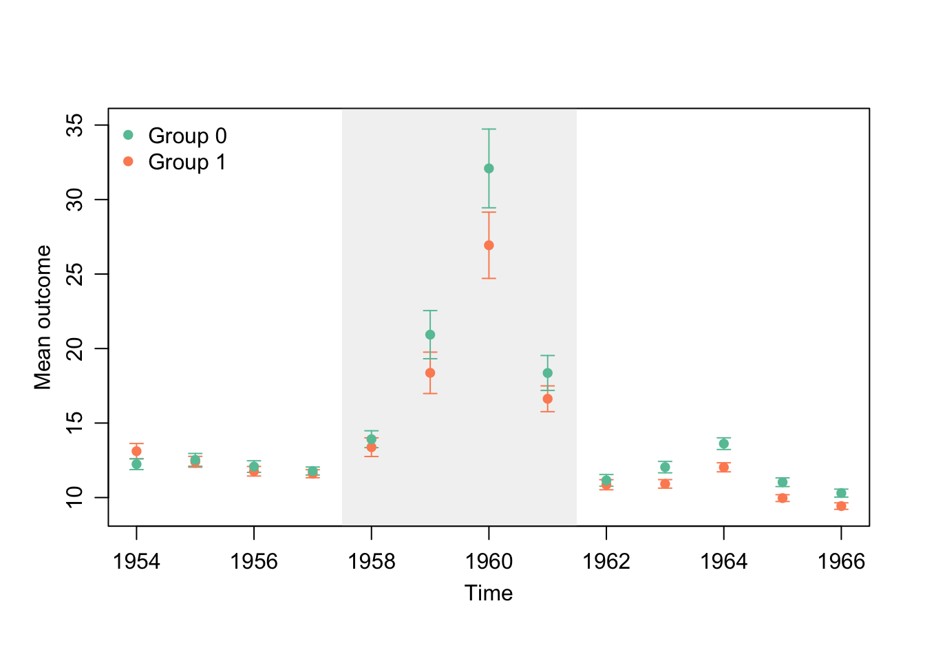
2.6.2 Dynamic estimates
Use type = "dynamic" to plot period-by-period estimates relative to the reference period. These estimates come from separate cross-sectional estimations by year, not a single TWFE event-study regression.
plot(fdid_results_ols1, type = "dynamic")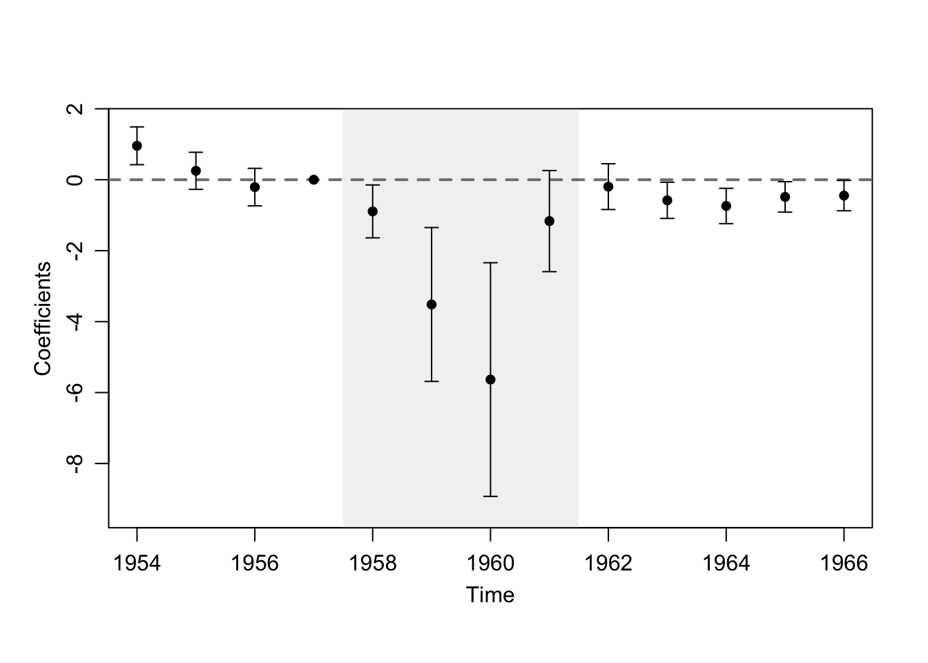
2.6.3 Diagnostic test for overlap
For method = "ipw" and method = "aipw", the user can assess the overlap assumption using type = "overlap", which plots the propensity score distributions by group.
plot(fdid_results_aipw, type = "overlap")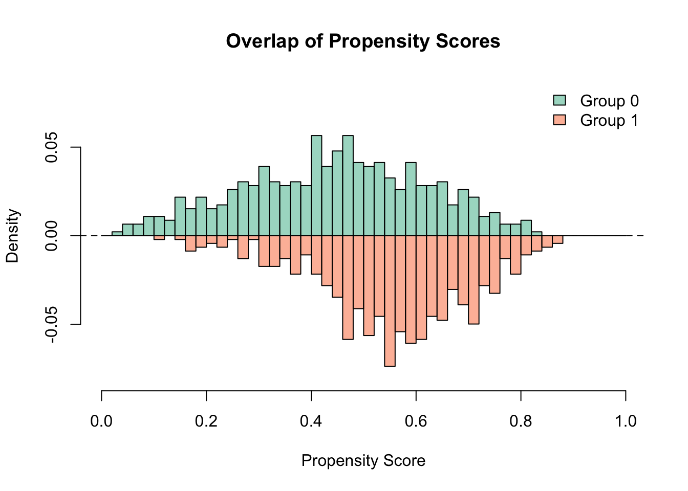
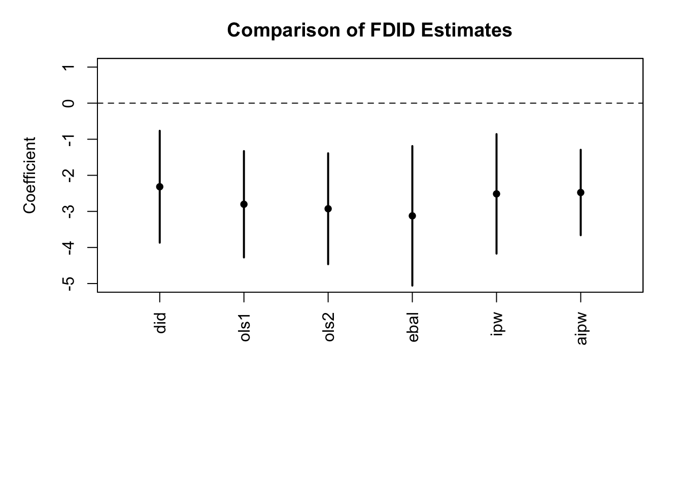
2.6.4 Comparison of methods
Use fdid_list() to collect multiple fdid() results and plot them together. The plot shows point estimates and 95% confidence intervals for each method.