4  LCS Female Samples

In this section, We report findings using the LaLonde female samples reconstructed by Calónico and Smith (2017), referred to as the LaLonde-Calónico-Smith (LCS) sample.

4.1 Prepare the Data

Consistent with LaLonde’s original analysis, the outcome variable is earnings in 1979 (re79). We use the same set of covariates as in LaLonde. Notably, this set does not include two pretreatment variables: earnings in 1974 and employment status in 1974. We also exclude the number of children in 1975 (nchildren75), which is available in the LCS dataset, from the covariates so that it can serve as a placebo outcome.

Code

# source the functions provided in part 1
source("https://github.com/xuyiqing/lalonde/blob/main/tutorial/functions.R?raw=TRUE")

Code

load("data/lcs.RData")

# expc = 0: experimental treated; 
# expc = 1: experimental control; 
# expc = 2: psid control.

lcs_psid$expc <- 0 
lcs_psid[lcs_psid$treat==0, ]$expc <- 2 
lcs_tr <- lcs[lcs$treat==1, ]
lcs_co <- lcs[lcs$treat==0, ]
lcs_co$treat <-  1
lcs_co$expc <- 1
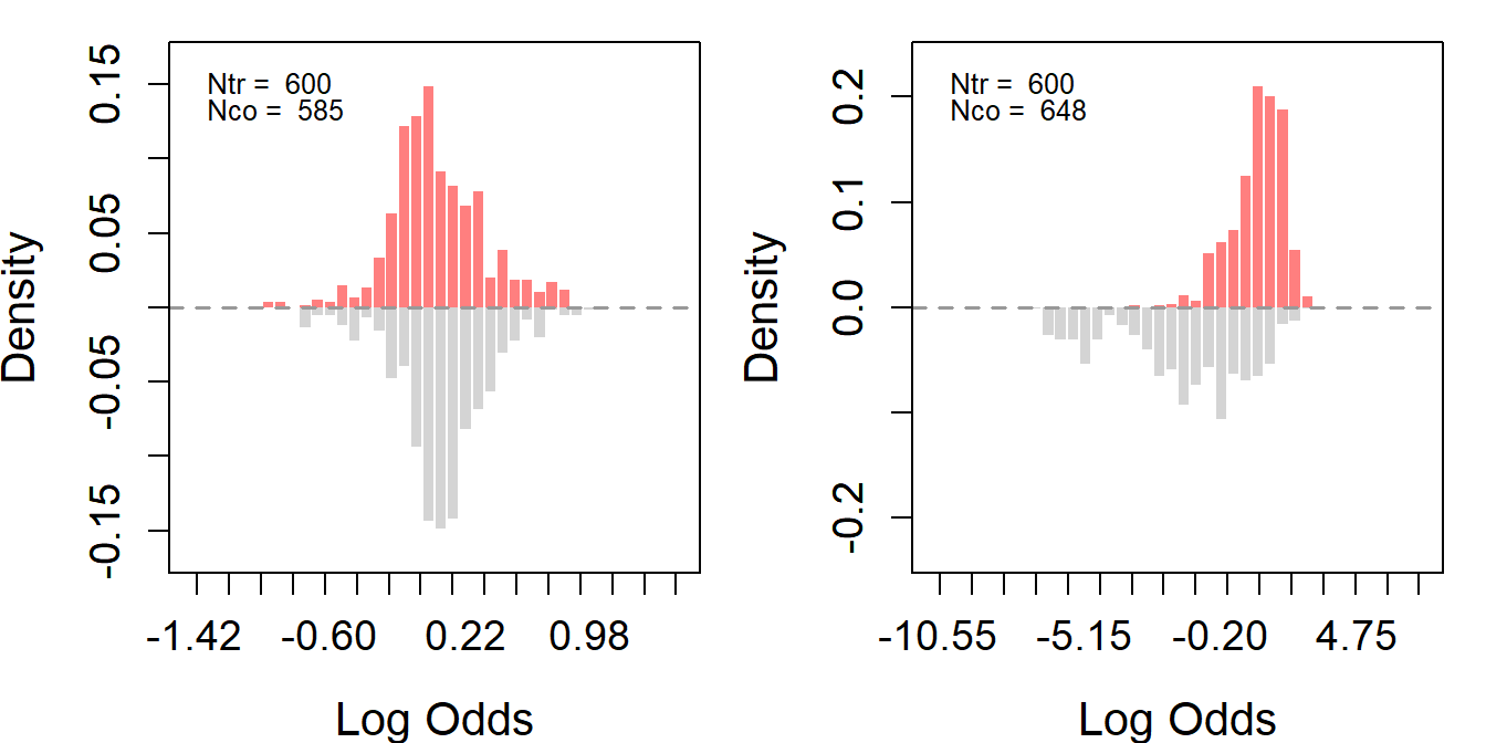
lcs_psid.plus <- rbind.data.frame(lcs_psid, lcs_co)

4.2 Assessing Overlap

We assess overlap in covariate distributions between treated and control groups based on the propensity score via GRF (log odds ratio) for the LCS-Experimental and LCS-PSID data.

Code

# define variables
Y <- "re79"
treat <- "treat"
# redifine covariates: removing "nchildren75" to be used as placebo outcome
covar <- c("age", "educ", "nodegree", "married", "black", "hisp", "re75", "u75")

4.2.1 LCS-Experimental and LCS-CPS1

Figure B10 demonstrates overlap in the LDW using the propensity score estimated via GRF (log odds ratio).

Code

par(mfrow = c(1,2))
lcs_ps <- assess_overlap(data = lcs, treat = treat, cov = covar, xlim = c(-1.5, 1.5), breaks = 40)
lcs_psid_ps <- assess_overlap(data = lcs_psid, treat = treat, cov = covar, xlim = c(-11, 7), breaks = 40)

FIGURE B10 (SM). Subfigure A: LCS-Experimental. Subfigure B: LCS-PSID.

4.3 Trimming to Improve Overlap

We then trim the data to improve overlap in covariate distributions by removing units with poor overlap based on the propensity score. This step aims to refine the datasets to improve later causal inference. With the trimmed data, we can reassess overlap for each group.

Like before, we start by assessing overlaps between the distributions of the treated and control groups based on log-odds derived from propensity scores.

Code

lcs_psid.plus_ps <- assess_overlap(data = lcs_psid.plus, treat = treat, cov = covar, xlim = c(-15, 5))

Then, we proceed with trimming to improve the quality of the causal inference. After trimming, we would expect the distributions to align more closely - the treatment and control groups are more comparable according to their covariates.

Code

trim <- function(data, ps = "ps_assoverlap", threshold = 0.9) {
  sub <- data[which(data[, ps] < threshold), ]
  return(sub)
}

#Trim
lcs_psid_trim <- trim(lcs_psid.plus_ps, threshold = 0.9)

# psid data: excluding the experimental controls
lcs_psid_trim_match <- subset(lcs_psid_trim, expc %in% c(0, 2) & ps_assoverlap)
# re-estimate propensity scores and employ 1:1 matching
lcs_psid_trim_match <- psmatch(data = lcs_psid_trim_match, Y = "re79", treat = "treat", cov = covar)

Code

#psid: trim experimental data
lcs_trim_psid <- subset(lcs_psid_trim, expc %in% c(0, 1))
lcs_trim_psid$treat[which(lcs_trim_psid$expc == 1)] <- 0

4.4 Reassessing Overlap

The propensity scores are reestimated after trimming.The plots below show good overlaps especially in the center, indicating an improved balance and common support between the treated and control groups. The before-after trimming comparison suggests that the trim effectively removes units that were less comparable.

Code

# psid data
lcs_psid_trim_match_ps <- assess_overlap(data = lcs_psid_trim_match, treat = treat, cov = covar, xlim = c(-3,3), breaks = 40)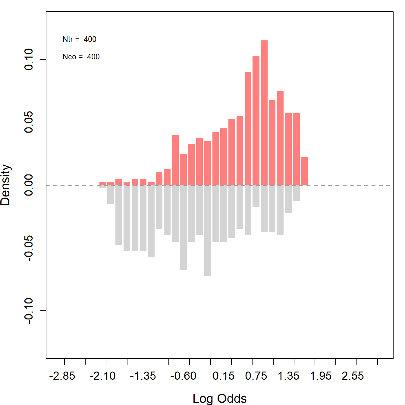

FIGURE B10 (SM). Subfigure C: Trimmed LCS-PSID.

4.5 Checking Covariate Balance

We can also check covariate balance directly by love.plot().

Code

load("data/lcs.RData")
# psid data
love.plot(lcs_psid, lcs_psid_trim_match, treat = treat, covar = covar, title = "Covariate Balance of LCS-PSID1")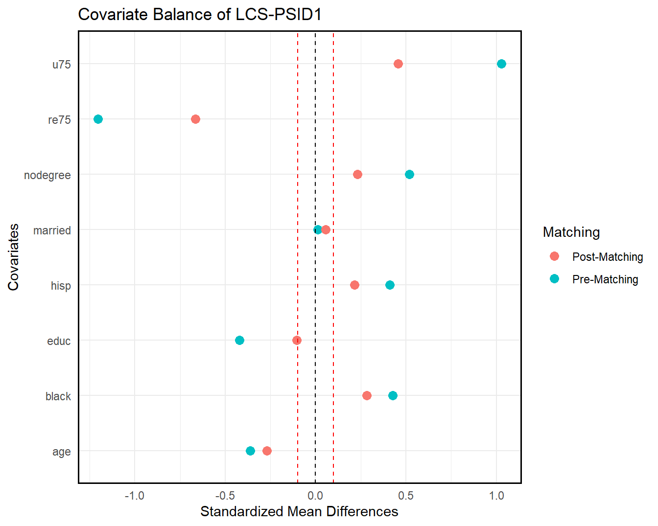

4.6 Estimating the ATT

Table B6 shows the ATT estimates using the reconstructed LaLonde female samples. Reconstructed PSID-1 is used as the nonexperimental control group. Figure B11 visualizes the ATT estimates.

Using the LCS female samples, we find that many modern methods yield estimates close to the experimental benchmarks, though standard errors are often quite large.

Code

set.seed(1234)
load("data/lcs.RData") 
# experimental
out1 <- estimate_all(lcs, Y, "treat", covar)
out2 <- estimate_all(lcs_trim_psid, Y, "treat", covar)
# no experimental
out3 <- estimate_all(lcs_psid, Y, "treat", covar)
out4 <- estimate_all(lcs_psid_trim, Y, "treat", covar)

Code

# print the result
a <- list(out3, out4)
# columns are samples
n <- nrow(out1) + 1   # add experimental benchmark
sav <- matrix("", n, length(a)*3-1)
for (j in 1:length(a)) {
    out <- a[[j]]
    for (i in 1: (n-1)) {
        sav[i+1, j*3-2] <- sprintf("%.0f", out[i, 1])
        sav[i+1, j*3-1] <- paste0("(", sprintf("%.0f", out[i, 2]), ")")    
    }
}
sav[1, 1] <- sprintf("%.0f", out1[1, 1]) # full experimental
sav[1, 4] <- sprintf("%.0f", out2[1, 1]) # trimmed experimental (PSID)
sav[1, 2] <- paste0("(", sprintf("%.0f", out1[1, 2]), ")")    
sav[1, 5] <- paste0("(", sprintf("%.0f", out2[1, 2]), ")")    
colnames(sav) <- c("LCS-PSID", "", "", "LCS-PSID (PS Trimmed)", "")
rownames(sav) <- c("Experimental Benchmark", "Difference-in-Means", "Regression", " Oaxaca Blinder", "GRF", "NN Matching", "PS Matching", "IPW", "CBPS", "Entropy Balancing", "DML-ElasticNet", "AIPW-GRF")
sav %>% knitr::kable(booktabs=TRUE, caption = "TABLE B6 in the Supplementary Materials (SM), ATT Estimates: Reconstructed LaLonde Female Samples")

TABLE B6 in the Supplementary Materials (SM), ATT Estimates: Reconstructed LaLonde Female Samples

	LCS-PSID			LCS-PSID (PS Trimmed)
Experimental Benchmark	821	(308)		785	(380)
Difference-in-Means	-4172	(412)		-804	(422)
Regression	808	(389)		359	(414)
Oaxaca Blinder	1128	(239)		608	(296)
GRF	918	(238)		395	(296)
NN Matching	1037	(531)		443	(519)
PS Matching	872	(333)		364	(402)
IPW	1043	(468)		506	(459)
CBPS	1217	(429)		670	(435)
Entropy Balancing	1229	(430)		673	(436)
DML-ElasticNet	814	(388)		411	(410)
AIPW-GRF	1050	(487)		424	(460)

Code

par(mfrow = c(2,1))
band <- out1[1, 3:4]
est <- out1[1, 1]
plot_coef(out3, band = band, line = est, ylim = c(-6000, 6000), main = "(A) LCS-PSID")

band <- out2[1, 3:4]
est <- out2[1, 1]
plot_coef(out4, band = band, line = est, ylim = c(-6000, 6000), main = "(B) Trimmed LCS-PSID")

FIGURE B11. ATT Estimates: Reconstructed LaLonde Female Sample

4.7 Alternative Estimands: CATT and QTET

4.7.1 Conditional Average Treatment Effect on the Treated (CATT)

The figures below show the CATT estimates using the reconstructed LaLonde female samples.

Each point on the scatter plots represents a pair of CATT estimates for a single unit: one from the experimental benchmark and one from the observational method. Points that lie on the 45-degree line (the red line) are cases where the observational and experimental methods yield the same estimate.

Code

# estimate catt
catt.lcs <- catt(lcs, Y, treat, covar)
catt.lcs.psid <- catt(lcs_trim_psid, Y, treat, covar) # trimmed experimental data
catt.psid <- catt(lcs_psid, Y, treat, covar)
catt.psid.trim <- catt(lcs_psid_trim, Y, treat, covar)

Code

par(mfrow = c(1,2))
# plot catt - "CATT (Experimental)" and "CATT (PSID-Full)"
par(mar = c(4, 4, 1, 1))
catt1 <- catt.lcs$catt
att1 <- catt.lcs$att[1]
catt2 <- catt.psid$catt
att2 <- catt.psid$att[1]
plot_catt(catt1, catt2, att1, att2, "CATT (Experimental)", "CATT (PSID-Full)",
    main = "", c(-8000, 8000))

# plot catt - "CATT (Experimental)" and "CATT (PSID-Trimmed)"
par(mar = c(4, 4, 1, 1))
catt1 <- catt.lcs.psid$catt
att1 <- catt.lcs.psid$att[1]
catt2 <- catt.psid.trim$catt
att2 <- catt.psid.trim$att[1]
plot_catt(catt1, catt2, att1, att2, "CATT (Experimental)", "CATT (PSID-Trimmed)",
    main = "", c(-8000, 8000))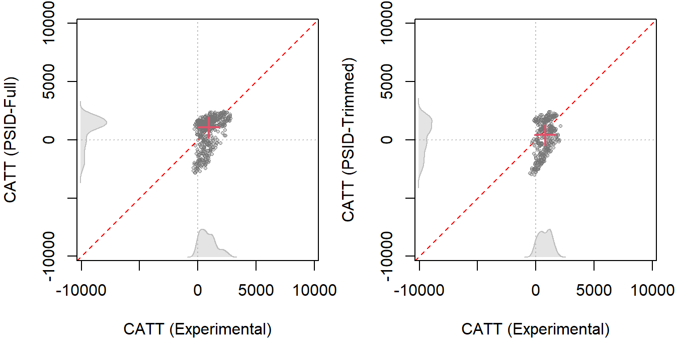

FIGURE B12. CATT Estimates for the reconstructed LaLonde female samples

Note: Scatterplots show the CATT using both experimental data (x-axis) and nonexperimental data (y-axis) from the reconstructed LaLonde female samples. Each dot corresponds to a CATT estimate based on the covariate values of a treated unit, while each red cross symbolizes the ATT estimates. For every estimate, the AIPW estimator is employed, with the GRF approach for estimating nuisance parameters. Different subfigures indicate various data comparisons: Subfigure A: Compares LCS-Experimental with LaLonde-PSID1. Subfigure B: Compares Trimmed LCS-Experimental to Trimmed LCS-PSID.

4.7.2 Quantile Treatment Effect on the Treated (QTET)

The Figures below show the quantile treatment effects on the treated in reconstructed LaLonde female samples. QTET analysis helps us to see where along the outcome distribution the treatment is more or less effective.

Code

# estimate qte (some of the following lines are not run due to computational limitation)
## experimental
qte.lcs <- est_qte(Y, treat, NULL, data = lcs)
qte.lcs.psid <- est_qte(Y, treat, NULL, data = lcs_trim_psid)
## non-experimental
qte.lcs_psid <- est_qte(Y, treat, covar, data = lcs_psid) # adjusted
qte.lcs_psid0 <- est_qte(Y, treat, NULL, data = lcs_psid) # unadjusted
qte.lcs_psid.trim <- est_qte(Y, treat, covar, data = lcs_psid_trim) # adjusted
qte.lcs_psid.trim0 <- est_qte(Y, treat, NULL, data = lcs_psid_trim) # unadjusted

Code

# plot qte
par(mfrow = c(1,2))

# PSID
plot_qte(qte.lcs_psid, qte.lcs_psid0, qte.lcs, main = "LCS-PSID", ylim = c(-25000, 15000))
legend("bottomleft", legend = c("Experimental", "Unadjusted", "Adjusted"), 
    lty = 1, pch = c(16, 17, 16), col = c(4, 2, 1), bty = "n")

# PSID trimmed
plot_qte(qte.lcs_psid.trim, qte.lcs_psid.trim0, qte.lcs.psid, main = "LCS-PSID (Trimmed)", ylim = c(-25000, 15000))
legend("bottomleft", legend = c("Experimental", "Unadjusted", "Adjusted"), 
    lty = 1, pch = c(16, 17, 16), col = c(4, 2, 1), bty = "n")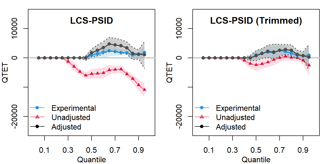

FIGURE B13: Quantile Treatment Effects: Reconstructed Female Samples

Note: Figures show the quantile treatment effects on the treated (QTET) using the reconstructed LaLonde female samples. Results from the experimental data are shown in blue and results from the nonexperimental data are shown in red for raw estimates and black for covariate-adjusted estimates. Each dot corresponds to a QTET estimate at a particular quantile, while shaded areas represent bootstrapped 95% confidence intervals. Unadjusted models do not incorporate covariates while adjustment models use the full set of covariates to estimate the propensity scores with a logit.

4.8 Placebo Tests

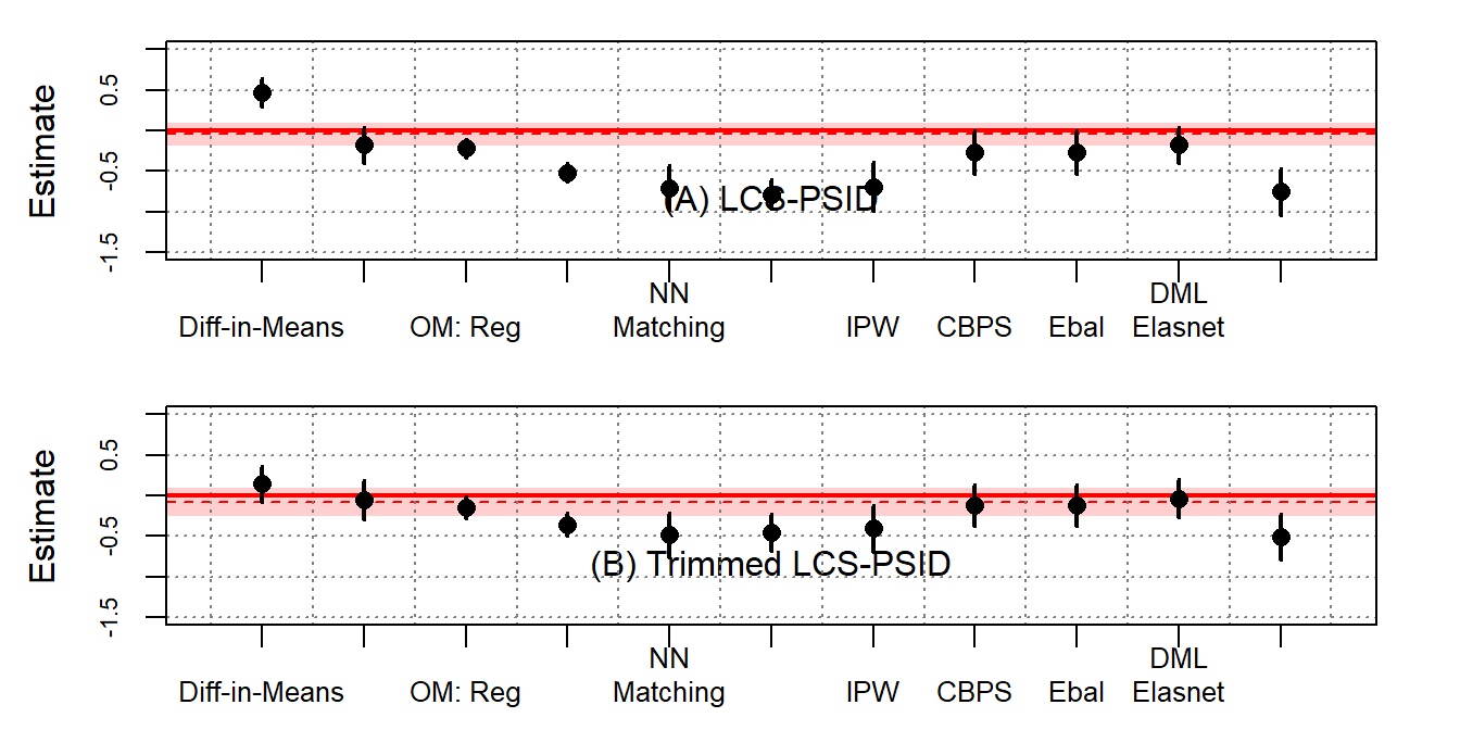
We conduct placebo analyses to further assess the plausibility of unconfoundedness. In the placebo analysis, estimators using observational data usually generate negative estimates. we fail to substantiate the unconfoundedness assumption with a placebo test using the number of children in 1975, a variable absent in LaLonde, as the placebo outcome.

Code

Y <- "nchildren75"
treat <- "treat"
covar <- c("age", "educ", "nodegree", "married", "black", "hisp", "re75", "u75")


set.seed(1234)
# experimental
out1 <- estimate_all(lcs, Y, "treat", covar)
out2 <- estimate_all(lcs_trim_psid, Y, "treat", covar)
# no experimental
out3 <- estimate_all(lcs_psid, Y, "treat", covar)
out4 <- estimate_all(lcs_psid_trim, Y, "treat", covar)

Code

# print the result
a <- list(out3, out4)
# columns are samples
n <- nrow(out1) + 1   # add experimental benchmark
sav <- matrix("", n, length(a)*3-1)
for (j in 1:length(a)) {
    out <- a[[j]]
    for (i in 1: (n-1)) {
        sav[i+1, j*3-2] <- sprintf("%.2f", out[i, 1])
        sav[i+1, j*3-1] <- paste0("(", sprintf("%.2f", out[i, 2]), ")")    
    }
}
sav[1, 1] <- sprintf("%.2f", out1[1, 1]) # full experimental
sav[1, 4] <- sprintf("%.2f", out2[1, 1]) # trimmed experimental (PSID)
sav[1, 2] <- paste0("(", sprintf("%.2f", out1[1, 2]), ")")    
sav[1, 5] <- paste0("(", sprintf("%.2f", out2[1, 2]), ")")    
colnames(sav) <- c("LCS-PSID", "", "", "LCS-PSID (PS Trimmed)", "")
rownames(sav) <- c("Experimental Benchmark", "Difference-in-Means", "Regression", " Oaxaca Blinder", "GRF", "NN Matching", "PS Matching", "IPW", "CBPS", "Entropy Balancing", "DML-ElasticNet", "AIPW-GRF")
sav %>% knitr::kable(booktabs=TRUE, caption = "TABLE B7 in the Supplementary Materials (SM): Placebo Test: Number of Children in 1975 as the Outcome")

TABLE B7 in the Supplementary Materials (SM): Placebo Test: Number of Children in 1975 as the Outcome

	LCS-PSID			LCS-PSID (PS Trimmed)
Experimental Benchmark	-0.05	(0.08)		-0.08	(0.09)
Difference-in-Means	0.47	(0.09)		0.14	(0.11)
Regression	-0.18	(0.11)		-0.05	(0.12)
Oaxaca Blinder	-0.22	(0.06)		-0.15	(0.07)
GRF	-0.52	(0.06)		-0.36	(0.07)
NN Matching	-0.71	(0.14)		-0.49	(0.14)
PS Matching	-0.79	(0.09)		-0.46	(0.12)
IPW	-0.69	(0.15)		-0.41	(0.15)
CBPS	-0.27	(0.14)		-0.12	(0.13)
Entropy Balancing	-0.27	(0.14)		-0.12	(0.13)
DML-ElasticNet	-0.18	(0.11)		-0.03	(0.12)
AIPW-GRF	-0.75	(0.15)		-0.51	(0.14)

Code

par(mfrow = c(2,1))
band <- out1[1, 3:4]
est <- out1[1, 1]
plot_coef(out3, band = band, line = est, ylim = c(-1.5, 1), main = "(A) LCS-PSID")

band <- out2[1, 3:4]
est <- out2[1, 1]
plot_coef(out4, band = band, line = est, ylim = c(-1.5, 1), main = "(B) Trimmed LCS-PSID")

FIGURE B14. Placebo Test: Number of Children in 1975 as the Outcome

4.9 Sensitivity Analyses

Below are our sensitivity analyses using the reconstructed LaLonde female samples, with results depicted in contour plots below.

Code

par(mfrow = c(1,2))

# define variables
Y <- "re79"
treat <- "treat"
# redifine covariates: removing "nchildren75" to be used as placebo outcome
covar <- c("age", "educ", "nodegree", "married", "black", "hisp", "re75", "u75")
bm <- c("re75")

# LCS-Experimental data
sens_ana(lcs, Y, treat, covar, bm, kd = 1)

# trimmed LCS-PSID data
sens_ana(lcs_psid, Y, treat, covar, bm, kd = 1:3)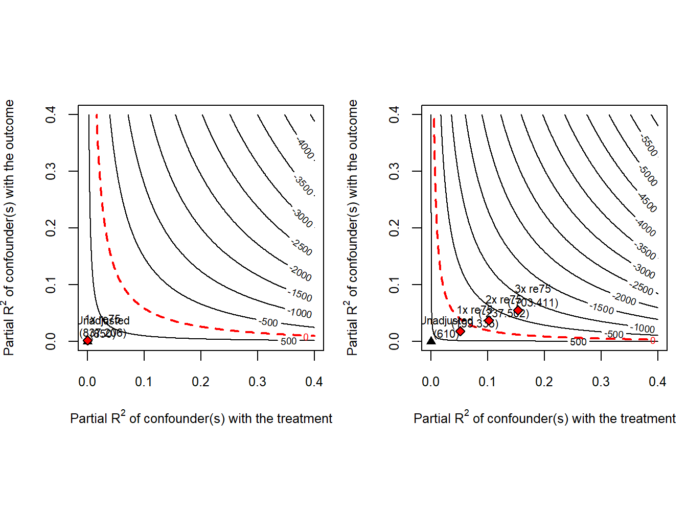

FIGURE B15. Sensitivity Analyses for Trimmed LDW-CPS and LDW-PSID

The analysis shows that the estimated training effect based on LCS-PSID is sensitive to potential confounders that behave like re75.

Calónico, Sebastian, and Jeffrey Smith. 2017. “The Women of the National Supported Work Demonstration.” Journal of Labor Economics 35 (S1): S65–97.

Dehejia, Rajeev H, and Sadek Wahba. 1999. “Causal Effects in Nonexperimental Studies: Reevaluating the Evaluation of Training Programs.” Journal of the American Statistical Association 94 (448): 1053–62.

———. 2002. “Propensity Score-Matching Methods for Nonexperimental Causal Studies.” Review of Economics and Statistics 84 (1): 151–61.

Firpo, Sergio. 2007. “Efficient Semiparametric Estimation of Quantile Treatment Effects.” Econometrica 75 (1): 259–76.

Imbens, Guido W, Donald B Rubin, and Bruce I Sacerdote. 2001. “Estimating the Effect of Unearned Income on Labor Earnings, Savings, and Consumption: Evidence from a Survey of Lottery Players.” American Economic Review, 778–94.

LaLonde, Robert J. 1986. “Evaluating the Econometric Evaluations of Training Programs with Experimental Data.” The American Economic Review, 604–20.